numpy常用函数2

numpy常用函数学习2

点乘法

该方法为数学方法，但是在numpy使用的时候略坑。numpy的点乘为a.dot(b)或numpy.dot(a,b)，要求a,b的原始数据结构为MxN .* NxL=MxL，不是显示数据，必须经过a.resize()或者a.shape=两种方法转换才能将原始数据改变结构。
代码如下：

>>> import numpy as np
>>> a=np.array([[1,2,3,4],[5,6,7,8]])
>>> a
array([[1, 2, 3, 4],
       [5, 6, 7, 8]])
>>> b=np.array([[9],[9]])
>>> b
array([[9],
       [9]])
>>> a*b
array([[ 9, 18, 27, 36],
       [45, 54, 63, 72]])
>>> a.dot(b)
Traceback (most recent call last):
  File "<pyshell#6>", line 1, in <module>
    a.dot(b)
ValueError: shapes (2,4) and (2,1) not aligned: 4 (dim 1) != 2 (dim 0)
>>> c=np.array([[9],[10]])
>>> a*c
array([[ 9, 18, 27, 36],
       [50, 60, 70, 80]])
>>> d=np.array([[10,20,30,40],[50,60,70,80]])
>>> a.dot(d)
Traceback (most recent call last):
  File "<pyshell#10>", line 1, in <module>
    a.dot(d)
ValueError: shapes (2,4) and (2,4) not aligned: 4 (dim 1) != 2 (dim 0)

>>> d.reshape(4,2)
array([[10, 20],
       [30, 40],
       [50, 60],
       [70, 80]])
>>> a.dot(d)
Traceback (most recent call last):
  File "<pyshell#23>", line 1, in <module>
    a.dot(d)
ValueError: shapes (2,4) and (2,4) not aligned: 4 (dim 1) != 2 (dim 0)
>>> d
array([[10, 20, 30, 40],
       [50, 60, 70, 80]])
>>> d.resize(4,2)
>>> a.dot(d)
array([[ 500,  600],
       [1140, 1400]])
>>> a
array([[1, 2, 3, 4],
       [5, 6, 7, 8]])
>>> e=np.array([7,8,9,10])
>>> e.shape=(4,1)
>>> a.dot(e)
array([[ 90],
       [226]])

线型预测

通过最小二乘法对已有数据拟合出函数，并预测未知数据。
最小二乘法：在假定函数结构(这里假设我们知道结果是y=ax+b)的情况下，通过已知结果(x,y)求取未知变量(a,b)。
具体求取原理参考：https://baijiahao.baidu.com/s?id=1613474944612061421&wfr=spider&for=pc
预测例子：

import datetime as dt
import numpy as np
import pandas as pd
import matplotlib.pyplot as mp
import matplotlib.dates as md


def dmy2ymd(dmy):
    dmy = str(dmy, encoding='utf-8')
    date = dt.datetime.strptime(dmy, '%d-%m-%Y').date()
    ymd = date.strftime('%Y-%m-%d')
    return ymd

dates, closing_prices = np.loadtxt(
    '../../data/aapl.csv', delimiter=',',
    usecols=(1, 6), unpack=True,
    dtype='M8[D], f8', converters={1: dmy2ymd})
N = 5
pred_prices = np.zeros(
    closing_prices.size - 2 * N + 1)
for i in range(pred_prices.size):
    a = np.zeros((N, N))
    for j in range(N):
        a[j, ] = closing_prices[i + j:i + j + N]
    b = closing_prices[i + N:i + N * 2]
    #[1]挤后面的为残差
    x = np.linalg.lstsq(a, b)[0]
    pred_prices[i] = b.dot(x)
mp.figure('Linear Prediction',
          facecolor='lightgray')
mp.title('Linear Prediction', fontsize=20)
mp.xlabel('Date', fontsize=14)
mp.ylabel('Price', fontsize=14)
ax = mp.gca()
# 设置水平坐标每个星期一为主刻度
ax.xaxis.set_major_locator(md.WeekdayLocator(
    byweekday=md.MO))
# 设置水平坐标每一天为次刻度
ax.xaxis.set_minor_locator(md.DayLocator())
# 设置水平坐标主刻度标签格式
ax.xaxis.set_major_formatter(md.DateFormatter(
    '%d %b %Y'))
mp.tick_params(labelsize=10)
mp.grid(linestyle=':')
dates = dates.astype(md.datetime.datetime)
mp.plot(dates, closing_prices, 'o-', c='lightgray',
        label='Closing Price')
dates = np.append(dates,
                  dates[-1] + pd.tseries.offsets.BDay())
mp.plot(dates[2 * N:], pred_prices, 'o-',
        c='orangered', linewidth=3,
        label='Predicted Price')
mp.legend()
mp.gcf().autofmt_xdate()
mp.show()

线性拟合

原理同上：通过最小二乘法对已有数据拟合出函数，并预测未知数据。

y`代表预测值
y-y`为误差
kx + b = y y`
kx1 + b = y1 y1`  (y1-y1`)^2
kx2 + b = y2 y2`  (y2-y2`)^2
...
kxn + b = yn  yn`  (yn-yn`)^2
----------------------------------------------------------
E=f(,k,b)
找到合适的k和b，使E取得最小，由此，k和b所确定的直线为拟合直线。
/ x1 1 \      / k \         / y1` \
| x2 1  | X | b | 接近 | y2` |
| ...      |     \    /        | ...   |
\ xn 1/                     \ yn`/
    a             x           b
    最小二乘法的方法：
                   = np.linalg.lstsq(a, b)[0]
y = kx + b
kx1 + b = y1' - y1
kx2 + b = y2' - y2
...
kxn + b = yn' - yn
[y1 - (kx1 + b)]^2 +
[y2 - (kx2 + b)]^2 + ... +
[yn - (kxn + b)]^2 = loss = f(k, b)
k, b? -> loss ->min

趋势线示例：

# -*- coding: utf-8 -*-
from __future__ import unicode_literals
import datetime as dt
import numpy as np
import matplotlib.pyplot as mp
import matplotlib.dates as md

def dmy2ymd(dmy):
    dmy = str(dmy, encoding='utf-8')
    date = dt.datetime.strptime(dmy, '%d-%m-%Y').date()
    ymd = date.strftime('%Y-%m-%d')
    return ymd
dates, opening_prices, highest_prices, \
    lowest_prices, closing_prices = np.loadtxt(
        r'C:\Users\Cs\Desktop\数据分析\DS+ML\DS\data\aapl.csv',
        delimiter=',', usecols=(1, 3, 4, 5, 6),
        unpack=True, dtype='M8[D], f8, f8, f8, f8',
        converters={1: dmy2ymd})
trend_points = (highest_prices+lowest_prices+closing_prices)/3
days = dates.astype(int)
# =np.column_stack：将一位矩阵以纵向组合
"""
>>> a=[1,2,3];b=[11,22,33];np.column_stack((a,b))
array([[ 1, 11],
       [ 2, 22],
       [ 3, 33]])
"""
# 同理还有row_stack()，方法与其刚好相反
# np.ones_like() 生成一个与参数矩阵结构相同但值为1的矩阵
a = np.column_stack((days, np.ones_like(days)))
# 生成a,b的组合,暂时不知道多个变量情况下的拟合的公示，查手册
x = np.linalg.lstsq(a, trend_points)[0]
#print(np.linalg.lstsq(a, trend_points))
# ：(array([ 1.81649663e-01, -2.37829793e+03]), array([1267.18780684]), 2, array([8.22882234e+04, 4.62700411e-03]))
#得到的y`的值矩阵
trend_line = days*x[0]+x[1]
mp.figure('Candlestick', facecolor='lightgray')
mp.title('Candlestick', fontsize=20)
mp.xlabel('Date', fontsize=14)
mp.ylabel('Price', fontsize=14)
ax = mp.gca()
# 设置水平坐标每个星期一为主刻度
ax.xaxis.set_major_locator(md.WeekdayLocator(
    byweekday=md.MO))
# 设置水平坐标每一天为次刻度
ax.xaxis.set_minor_locator(md.DayLocator())
# 设置水平坐标主刻度标签格式
ax.xaxis.set_major_formatter(md.DateFormatter(
    '%d %b %Y'))
mp.tick_params(labelsize=10)
mp.grid(linestyle=':')
dates = dates.astype(md.datetime.datetime)
# 阳线掩码
rise = closing_prices - opening_prices >= 0.01
# 阴线掩码
fall = opening_prices - closing_prices >= 0.01
# 填充色
fc = np.zeros(dates.size, dtype='3f4')
fc[rise], fc[fall] = (1, 1, 1), (0, 0.5, 0)
# 边缘色
ec = np.zeros(dates.size, dtype='3f4')
ec[rise], ec[fall] = (1, 0, 0), (0, 0.5, 0)
mp.bar(dates, highest_prices - lowest_prices, 0,
       lowest_prices, color=fc, edgecolor=ec)
mp.bar(dates, closing_prices - opening_prices, 0.8,
       opening_prices, color=fc, edgecolor=ec)
mp.plot(dates, trend_line)
# 自动调整水平坐标轴的日期标签
mp.gcf().autofmt_xdate()
mp.show()

裁剪、压缩和累乘

ndarray.clip(min=下限, max=上限)
将调用数组中小于和大于下限和上限的元素替换为下限和上限，返回裁剪后的数组，调用数组保持不变。
ndarray.compress(条件)
返回由调用数组中满足条件的元素组成的新数组。
ndarray.prod()
返回调用数组中所有元素的乘积——累乘。
ndarray.cumprod()
返回调用数组中所有元素执行累乘的过程数组。

import numpy as np
a = np.array([10, 20, 30, 40, 50])
print(a)
b = a.clip(min=15, max=45)
print(b)
c = a.compress((15 <= a) & (a <= 45))
print(c)
d = a.prod()
print(d)
e = a.cumprod()
print(e)
def jiecheng(n):
    return n if n == 1 else n * jiecheng(n - 1)
n = 5
print(jiecheng(n))
jc = 1
for i in range(2, n + 1):
    jc *= i
print(jc)
print(np.arange(2, n + 1).prod())
结果：
[10 20 30 40 50]
[15 20 30 40 45]
[20 30 40]
12000000
[      10      200     6000   240000 12000000]
120
120
120

相关性

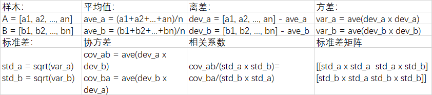
相关性：
相关系数=相关系数
cov_ab/(std_a x std_b)=cov_ba/(std_b x std_a)
协方差矩阵：

标准差矩阵：

相关性矩阵=协方差矩阵/标准差矩阵：（等号右边是一个矩阵）
| var_a/(std_a x std_a) cov_ab/(std_a x std_b) |
相关性= | cov_ba/(std_b x std_a) var_b/(std_b x std_b) |

numpy.cov(a, b)->相关矩阵的分子矩阵（协方差矩阵）
numpy.corrcoef(a, b)->相关性矩阵
手动和自动计算的例：

import datetime as dt
import numpy as np
import matplotlib.pyplot as mp
import matplotlib.dates as md

def dmy2ymd(dmy):
    dmy = str(dmy, encoding='utf-8')
    date = dt.datetime.strptime(
        dmy, '%d-%m-%Y').date()
    ymd = date.strftime('%Y-%m-%d')
    return ymd

dates, bhp_closing_prices = np.loadtxt(
    '../../data/bhp.csv', delimiter=',',
    usecols=(1, 6), unpack=True,
    dtype='M8[D], f8', converters={1: dmy2ymd})
vale_closing_prices = np.loadtxt(
    '../../data/vale.csv', delimiter=',',
    usecols=(6), unpack=True)
bhp_returns = np.diff(
    bhp_closing_prices) / bhp_closing_prices[:-1]
vale_returns = np.diff(
    vale_closing_prices) / vale_closing_prices[:-1]
ave_a = bhp_returns.mean()
dev_a = bhp_returns - ave_a
var_a = (dev_a * dev_a).sum() / (dev_a.size - 1)
std_a = np.sqrt(var_a)
ave_b = vale_returns.mean()
dev_b = vale_returns - ave_b
var_b = (dev_b * dev_b).sum() / (dev_b.size - 1)
std_b = np.sqrt(var_b)
cov_ab = (dev_a * dev_b).sum() / (dev_a.size - 1)
cov_ba = (dev_b * dev_a).sum() / (dev_b.size - 1)
#相关系数
corr = np.array([
    [var_a / (std_a * std_a), cov_ab / (std_a * std_b)],
    [cov_ba / (std_b * std_a), var_b / (std_b * std_b)]])
print(corr)
#相关性矩阵的分子矩阵：协方差矩阵
covs = np.cov(bhp_returns, vale_returns)
#相关性矩阵的分母矩阵：标准差矩阵
stds = np.array([
    [std_a * std_a, std_a * std_b],
    [std_b * std_a, std_b * std_b]])
corr = covs / stds
print(corr)
corr = np.corrcoef(bhp_returns, vale_returns)
print(corr)
mp.figure('Correlation Of Returns',
          facecolor='lightgray')
mp.title('Correlation Of Returns', fontsize=20)
mp.xlabel('Date', fontsize=14)
mp.ylabel('Returns', fontsize=14)
ax = mp.gca()
ax.xaxis.set_major_locator(md.WeekdayLocator(
    byweekday=md.MO))
ax.xaxis.set_minor_locator(md.DayLocator())
ax.xaxis.set_major_formatter(md.DateFormatter(
    '%d %b %Y'))
mp.tick_params(labelsize=10)
mp.grid(linestyle=':')
dates = dates.astype(md.datetime.datetime)
mp.plot(dates[:-1], bhp_returns, c='orangered',
        label='BHP')
mp.plot(dates[:-1], vale_returns, c='dodgerblue',
        label='VALE')
mp.legend()
mp.gcf().autofmt_xdate()
mp.show()
结果：
[[1.         0.67841747]
 [0.67841747 1.        ]]
[[1.         0.67841747]
 [0.67841747 1.        ]]
[[1.         0.67841747]
 [0.67841747 1.        ]]

结果解读：
在相关性矩阵中，主对角线上的元素是1，代表每个随机变量关于其自身一定是最强的正相关，辅助角上的元素为去除了分散性以后的净相关性指标–相关系数。相关系数介于[-1,1]，正负代表了相关性的方向，绝对值表示了相关性的强弱。

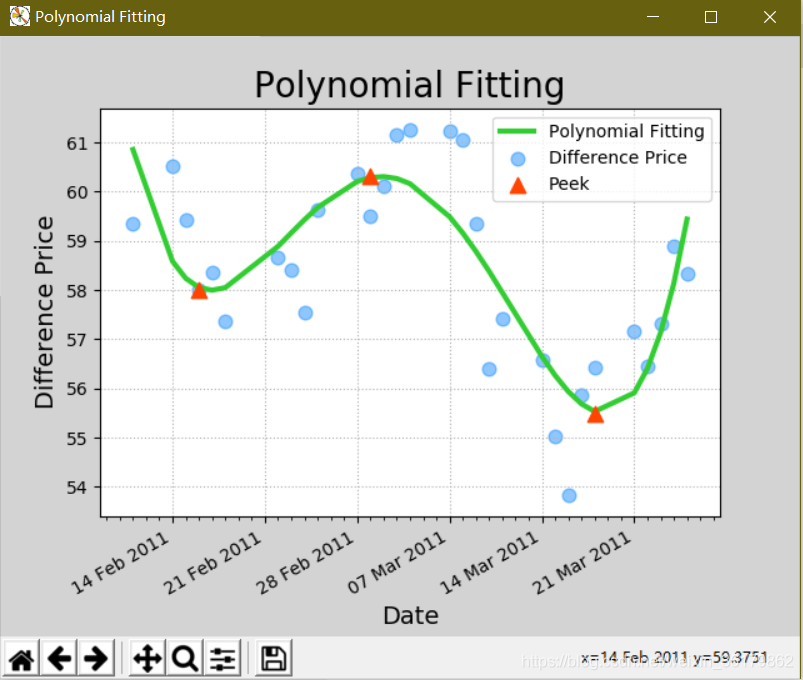
多项式拟合

y = p0x^n + p1x^n-1 + p2x^n-2 + … + pn = f(x)
y1’ = f(x1) -> y1
y2’ = f(x2) -> y2
…
yn’ = f(xn) -> yn
(y1-y1’)^2 + (y2-y2’)^2 + … + (yn-yn’)^2
= loss (p0, …, pn)
p0, …, pn = ? -> loss -> min
X = [x1, x2, …, xn] - 自变量
Y = [y1, y2, …, yn] - 实际函数值
Y’= [y1’,y2’,…,yn’] - 拟合函数值
P = [p0, p1, …, pn] - 多项式函数中的系数
Q = [q0, q1, …, qn-1] - 多项式函数导函数的系数
np.polyfit(X, Y, 最高次幂)->P
np.polyval(P, X)->Y’
np.polyder§->Q
y = 4x^3 + 3x^2 + 2x + 1, P=[4,3,2,1]
dy/dx = 12x^2 + 6x + 2, Q=[12, 6, 2]
4x^3 + 3x^2 + 2x + 1 = 0的根：np.roots§(f(x)=0的解)
np.polysub(P1, P2)->两个多项式函数的差函数的系数
y = 4x^3 + 3x^2 + 2x + 1, P1=[4,3,2,1]
y = 5x^4 + x, P2=[5, 0, 0, 1, 0]
y = -5x^4 + 4x^3 + 3x^2 + x + 1
np.polysub(P1, P2)->[-5, 4, 4, 1, 1]
np.polyfit(X, Y, 最高次幂)->P得到一个函数，赋予变量才可以得到值
np.roots§(f(x)=0的解)
np.polysub(P1, P2)->两个多项式函数的差函数的系数
np.polyval(p, days) 对曲线求值
【polyfit】多项式曲线拟合
【polyval】多项式曲线求值
np.polyder§对p函数求导、

# -*- coding: utf-8 -*-
from __future__ import unicode_literals
import datetime as dt
import numpy as np
import matplotlib.pyplot as mp
import matplotlib.dates as md


def dmy2ymd(dmy):
    dmy = str(dmy, encoding='utf-8')
    date = dt.datetime.strptime(
        dmy, '%d-%m-%Y').date()
    ymd = date.strftime('%Y-%m-%d')
    return ymd


dates, bhp_closing_prices = np.loadtxt(
    r'C:\Users\Cs\Desktop\数据分析\DS+ML\DS\data\bhp.csv', delimiter=',',
    usecols=(1, 6), unpack=True,
    dtype='M8[D], f8', converters={1: dmy2ymd})
vale_closing_prices = np.loadtxt(
    r'C:\Users\Cs\Desktop\数据分析\DS+ML\DS\data\vale.csv', delimiter=',',
    usecols=(6), unpack=True)
diff_closing_prices = bhp_closing_prices - vale_closing_prices
#将日期转换为int格式，方便计算
days = dates.astype(int)
print(dates)
# 拟合4次曲线
p = np.polyfit(days, diff_closing_prices, 4)
# 生成曲线定点的值
poly_closing_prices = np.polyval(p, days)
# 求导
q = np.polyder(p)
#解导数等于0的值
roots_x = np.roots(q)
#求导数等于0的时候函数值（y值）
roots_y = np.polyval(p, roots_x)
mp.figure('Polynomial Fitting', facecolor='lightgray')
mp.title('Polynomial Fitting', fontsize=20)
mp.xlabel('Date', fontsize=14)
mp.ylabel('Difference Price', fontsize=14)
ax = mp.gca()
ax.xaxis.set_major_locator(md.WeekdayLocator(
    byweekday=md.MO))
ax.xaxis.set_minor_locator(md.DayLocator())
ax.xaxis.set_major_formatter(md.DateFormatter(
    '%d %b %Y'))
mp.tick_params(labelsize=10)
mp.grid(linestyle=':')
dates = dates.astype(md.datetime.datetime)
mp.plot(dates, poly_closing_prices, c='limegreen',
        linewidth=3, label='Polynomial Fitting')
mp.scatter(dates, diff_closing_prices, c='dodgerblue',
           alpha=0.5, s=60, label='Difference Price')
#将求得的解转换为日期格式
roots_x = roots_x.astype(int).astype(
    'M8[D]').astype(md.datetime.datetime)
mp.scatter(roots_x, roots_y, marker='^', s=80,
           c='orangered', label='Peek', zorder=4)
mp.legend()
mp.gcf().autofmt_xdate()
mp.show()

提取符号数组

将数组的正负提取出来单独作为一个数组：
两种方法：

• np.sign(源数组)->符号数组
  + -> 1
  - -> -1
  0 -> 0
• np.piecewise(源数组, 条件序列, 取值序列)->目标数组
  针对源数组中的每一个元素，检测其是否符合条件序列中的每一个条件，符合哪个条件就用取值系列中与之对应的值，表示该元素，放到目标数组中返回。
  条件序列: [a < 0, a == 0, a > 0]
  取值序列: [-1, 0, 1]

# -*- coding: utf-8 -*-
from __future__ import unicode_literals
import numpy as np
a = np.array([70, 80, 60, 30, 40])
print(a)
b = a - 60
print(b)
c = np.sign(b)
print(c)
d = np.piecewise(a, [a < 60, a == 60, a > 60],[-1, 0, 1])
print(d)

例子2（没啥意义，和例子一差不多）：

# -*- coding: utf-8 -*-
from __future__ import unicode_literals
import datetime as dt
import numpy as np
import matplotlib.pyplot as mp
import matplotlib.dates as md


def dmy2ymd(dmy):
    dmy = str(dmy, encoding='utf-8')
    date = dt.datetime.strptime(
        dmy, '%d-%m-%Y').date()
    ymd = date.strftime('%Y-%m-%d')
    return ymd


dates, closing_prices, volumes = np.loadtxt(
    r'C:\Users\Cs\Desktop\数据分析\DS+ML\DS\data\bhp.csv', delimiter=',',
    usecols=(1, 6, 7), unpack=True,
    dtype='M8[D], f8, f8', converters={1: dmy2ymd})
diff_closing_prices = np.diff(closing_prices)
#sign_closing_prices = np.sign(diff_closing_prices)
sign_closing_prices = np.piecewise(
    diff_closing_prices, [
        diff_closing_prices < 0,
        diff_closing_prices == 0,
        diff_closing_prices > 0], [-1, 0, 1])
print(volumes)
obvs = volumes[1:] * sign_closing_prices
print(obvs)
mp.figure('On-Balance Volume', facecolor='lightgray')
mp.title('On-Balance Volume', fontsize=20)
mp.xlabel('Date', fontsize=14)
mp.ylabel('OBV', fontsize=14)
ax = mp.gca()
ax.xaxis.set_major_locator(md.WeekdayLocator(
    byweekday=md.MO))
ax.xaxis.set_minor_locator(md.DayLocator())
ax.xaxis.set_major_formatter(md.DateFormatter(
    '%d %b %Y'))
mp.tick_params(labelsize=10)
mp.grid(axis='y', linestyle=':')
dates = dates[1:].astype(md.datetime.datetime)
mp.bar(dates, obvs, 1.0, color='dodgerblue',
       edgecolor='white', label='OBV')
mp.legend()
mp.gcf().autofmt_xdate()
mp.show()

杂项

numpy.diff(a, n=1,axis=-1)
沿着指定轴计算第N维的离散差值
参数：
a：输入矩阵
n：可选，代表要执行几次差值
axis：默认是最后一个
示例：

>>> a=np.arange(2,14)
>>> a.shape=(3,4)
>>> a
array([[ 2,  3,  4,  5],
       [ 6,  7,  8,  9],
       [10, 11, 12, 13]])
>>> np.diff(a)
array([[1, 1, 1],
       [1, 1, 1],
       [1, 1, 1]])