Tensorflow框架（五）

本章是对前五章的总结

一、概述

Tensorflow框架的核心概念是计算图：

整个计算流图的主要包含以下几个部分：

导入数据
网络结构
损失函数
反向传播

由于Tensorflow框架的机制，反向传播过程并不需要我们去描述。因此我们要做的就是：

定义网络的结构
定义损失函数与反向传播算法
训练并测试模型

二、计算图

import tensorflow as tf
import numpy as np

# 定义常量
a = tf.constant([1.0], name = 'a')
b = tf.constant([2.0], name = 'b')
result = a + b
print(result)

输出结果：

# 定义常量
a = tf.constant([1.0], name = 'a')
b = tf.constant([2.0], name = 'b')
result = a + b

# 定义会话
with tf.Session() as sess:
    print(sess.run(result))

输出结果：

上述的代码定义了一个计算图，通过定义会话执行计算。可以形象地类比成一个管道系统，开始的时候我们只是构建了管道系统的结构与流通规则。但此时没有水流入，通过定义会话，将水通入管道系统，最后才能出现结果。

其中的a，b，result在tensorflow中都别称作张量（对运算结果的引用）

三、神经网络的搭建

在搭建神经网络之前，我们需要了解一下本次使用的数据集MNIST

MNSIT数据集是深度学习经典入门的demo，其训练集包含了55000张图片，验证集包含了5000张图片，测试集包含了10000张，其中每张图片是以28*28*1的矩阵形式存储

我们使用下面的代码来读取数据

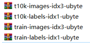
mnist = input_data.read_data_sets('./', one_hot = True)

这样会在当前文件夹下出现4个文件：

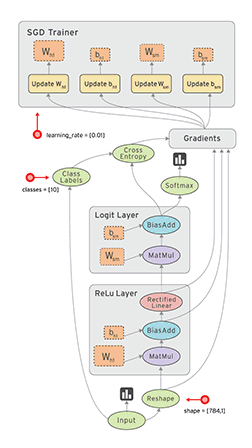
下面是一个简单的神经网络模型

基于此建立一个简单的神经网络：

import tensorflow as tf
from tensorflow.examples.tutorials.mnist import input_data
import numpy as np

# 使用下面语句在当前目录下下载并读取文件，如果文件已存在则直接读取
mnist = input_data.read_data_sets('./', one_hot = True)

# 每个批次的大小
batch_size = 100

# 定义两个placeholder,为数据的导入预留两个位置
# 这里的 None表示第一个维度暂时未知,在实际运行的时候会给定
x = tf.placeholder(tf.float32, [None, 784])
y = tf.placeholder(tf.float32, [None, 10])

# 这里的tf.matmul表示矩阵乘法
w1 = tf.Variable(tf.truncated_normal([784, 500], stddev = 0.1))
b1 = tf.Variable(tf.constant(0.1, shape = [500]))
a1 = tf.nn.relu(tf.matmul(x, w1) + b1)

w2 = tf.Variable(tf.truncated_normal([500,10], stddev = 0.1))
b2 = tf.Variable(tf.constant(0.1, shape = [10]))
logit = tf.nn.softmax(tf.matmul(a1, w2) + b2)

# 定义softmax损失函数
loss = tf.reduce_mean(tf.nn.sparse_softmax_cross_entropy_with_logits(
    logits = logit, labels = tf.argmax(y, 1)))

# 使用梯度下降法
train_step = tf.train.GradientDescentOptimizer(0.2).minimize(loss)

# 初始化变量
init = tf.global_variables_initializer()

# 将结果放在一个bool类型的列表中
# tf.argmax(y, 1) 表示按axis = 1,也就是按第二个维度取值最大的位置
correction_prediction = tf.equal(tf.argmax(y,1), tf.argmax(logit, 1))
# 求准确率
accuracy = tf.reduce_mean(tf.cast(correction_prediction, tf.float32))

# 定义会话
with tf.Session() as sess:
    sess.run(init)
    for i in range(20001):
        # 以100个样本作为一个批次
        start = (i * batch_size) % mnist.train.num_examples
        end = min(start + batch_size, mnist.train.num_examples)
        
        # 把当前批次的数据导入进神经网络
        sess.run(train_step,feed_dict = {x:mnist.train.images[start:end], y:mnist.train.labels[start:end]})
        if i % 1000 == 0:
            
            # 将训练集和测试集导入神经网络,计算准确率
            train_prediction = sess.run(accuracy, feed_dict = {x:mnist.train.images, y:mnist.train.labels})
            test_prediction = sess.run(accuracy, feed_dict = {x:mnist.test.images, y:mnist.test.labels})
            print("After %d, train correction: %g, test correction: %g" %(i, train_prediction, test_prediction))

运行结果：

四、优化算法

通过简单的搭建一个神经网络，我们可以了解到整个程序的大概面貌，但在实际使用情况中，需要对神经网络进行一些优化，以达到更好的预期效果。这里我们加入了正则化和学习率衰减优化算法。同时上面提到的代码从某种程度上来说，并不规范，因此添加优化算法后并进行规范化后的代码如下：

import tensorflow as tf
from tensorflow.examples.tutorials.mnist import input_data

input_node = 784 # mnist数据集共有28*28个像素，所以输入节点共有784
output_node = 10 # 输出层节点数
layer1_node = 500 # 隐藏层节点数
batch_size = 100 # 一个训练batch中的训练数据个数
learning_rate_base = 0.8 # 基础学习率
learning_rate_decay = 0.99 # 学习率衰减率
regularization_rate = 0.0001 # 正则化项
training_steps = 30000 # 训练轮数

def get_weight(shape, regularizer):
    '''
    如果有正则化项，则将weight加入到losses集合中
    '''
    weight = tf.get_variable('weight', shape, initializer = tf.truncated_normal_initializer(stddev = 0.1))
    if regularizer != None:
        tf.add_to_collection('losses', regularizer(weight))
    return weight

def get_bias(shape):
    bias = tf.get_variable('bias', shape, initializer = tf.constant_initializer(0.1))
    return bias

def inference(input_tensor, regularizer):
    '''
    神经网络正向传播过程
    '''
    # 对神经网络的第一层赋予名称layer1的命名空间
    with tf.variable_scope('layer1'):
        weight = get_weight([input_node, layer1_node], regularizer)
        tf.summary.histogram('weight1', weight)
        bias = get_bias([layer1_node])
        layer1 = tf.nn.relu(tf.matmul(input_tensor, weight) + bias)
        
    # 对神经网络的输出层赋予名称layer2的命名空间 
    with tf.variable_scope('layer2'):
        weight = get_weight([layer1_node, output_node], regularizer)
        tf.summary.histogram('weight2', weight)
        bias = get_bias([output_node])
        layer2 = tf.nn.softmax(tf.matmul(layer1, weight) + bias)
    return layer2


def train(mnist):
    # 定义输入空白位
    x = tf.placeholder(tf.float32, [None, input_node], name = 'x-input')
    y = tf.placeholder(tf.float32, [None, output_node], name = 'y-input')
    
    # 定义L2正则化项
    regularizer = tf.contrib.layers.l2_regularizer(regularization_rate)
    
    # 计算神经网络前向传播的结果
    logit = inference(x, regularizer)
    
    # 这里与之前说到滑动平均模型里的num_updates变量一致，通过模仿迭代次数来控制衰减速率
    global_step = tf.Variable(0, trainable = False)
    
    # 定义损失函数
    cross_entropy = tf.nn.sparse_softmax_cross_entropy_with_logits(
    logits = logit, labels = tf.argmax(y, 1))
    
    cross_entropy_mean = tf.reduce_mean(cross_entropy)
    
    # 总的损失等于交叉熵的损失和正则化损失的和
    loss = cross_entropy_mean + tf.add_n(tf.get_collection('losses'))
    
    # 学习率衰减函数
    learning_rate = tf.train.exponential_decay(
    learning_rate_base, # 基础学习率，在此基础上进行衰减
    global_step,        # 当前迭代的轮数
    mnist.train.num_examples, # 走完所有数据需要的迭代次数
    learning_rate_decay) # 学习率衰减速率
    
    # 使用梯度下降法优化
    train_step = tf.train.GradientDescentOptimizer(learning_rate).minimize(loss, global_step = global_step)
    
    # 测试输出结果是否与真实标签相等
    correction_prediction = tf.equal(tf.argmax(logit, 1), tf.argmax(y, 1))
    
    # 测试一组数据正确率
    # 这里将correction_pred类型改为tf.float32
    accuracy = tf.reduce_mean(tf.cast(correction_prediction, tf.float32))

    # 参数初始化
    init = tf.global_variables_initializer()
    
    with tf.Session() as sess:    
        sess.run(init)
        
        # 开始训练
        for i in range(training_steps):
            # 产生当前轮的训练批次
            xs, ys = mnist.train.next_batch(batch_size)
            sess.run(train_step, feed_dict = {x: xs, y:ys})
            
            # 每一千次训练测试一下验证集正确率
            if i % 1000 == 0:
                train_acc = sess.run(accuracy, feed_dict = {x: mnist.train.images, y: mnist.train.labels})
                
                test_acc= sess.run(accuracy, feed_dict = {x: mnist.test.images, y: mnist.test.labels})
                print("After %d training step, train accuracy is %g, test accuracy is %g" %(i, train_acc, test_acc))

# 执行程序
mnist = input_data.read_data_sets('./', one_hot = True)
tf.reset_default_graph()
train(mnist)

在tensorboard下，运行结果曲线图，这里的加粗线表示训练集精度，另外的线表示测试集精度。当迭代到一定程度时，曲线收敛。

五、卷积神经网络

对于简单的卷积神经网络，其结构如下图所示：

有了之前的基础，我们可以了解卷积神经网络的搭建。首先一般的卷积网络主要有：

卷积层
池化层
全连接层

其中全连接层与我们之前介绍的网络一样

首先是卷积层：这里的第一个和第二个维度表示了过滤器的尺寸，第三个维度表示了当前输入图层也就是上层的输出的通道数，第四个维度表示了过滤器的个数。

回顾一下卷积层的操作：

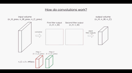
根据上面的图示看，

# 定义过滤器的权重
filter_weight = tf.get_variable('weight', [5,5,3,16], initializer = tf.truncated_normal_initializer(stddev = 0.1))

# 定义过滤器的偏置
bias = tf.get_variable('biases', [16], initializer = tf.truncated_normal_initializer(0.1))

之后我们定义卷积层运算：

conv = tf.nn.conv2d(input, filter_weight, strides = [1,1,1,1], padding = 'SAME')

这里的步长由于支队矩阵的长和宽有效，因此第一维和最后一维的一定为1

padding = 'SAME'表示用0填充，padding = 'VALID'表示不填充

设原图像尺寸为W * W，步长为s，过滤器尺寸为f * f，则经过卷积运算后的图像尺寸：

VALID： $\left \lceil (W-f+1) / s \right \rceil$

SAME： $\left \lceil W / s \right \rceil$

池化层又分成最大池化层和平均池化层：

# 最大池化层
# ksize维度里第一个和第四个必须为1，第二个和第三个维度表示过滤器尺寸
pool = tf.nn.max_pool(actived_conv, ksize = [1,3,3,1],
                      strides = [1,2,2,1], padding = 'SAME')
# 平均池化层
pool = tf.nn.avg_pool(actived_conv, ksize = [1,3,3,1],
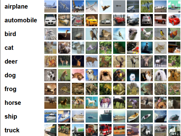
                      strides = [1,2,2,1], padding = 'SAME')

下面使用cifar-10数据集，cifar-10数据集总共有60000张彩色图像，50000张用于训练，另外10000张用于测试。其中每张图像是32*32*3规格的。共有10个类别，每个类别有5000张

使用VGGNet网络将会带来较好的效率，但也会因此产生巨大的时间开销，因此这里我们使用一个简化版的VGG-16网络对图像进行识别：

import tensorflow as tf
import numpy as np
import pickle

# 读取cifar-10数据集
def load_CIFAR_batch(filename):
    with open(filename, 'rb') as f:
        datadict = pickle.load(f,encoding='latin1')
        X = datadict['data']
        Y = datadict['labels']
        X = X.reshape(10000, 3, 32,32).transpose(0,2,3,1).astype("float")
        Y = np.array(Y)
        return X, Y

# 给定文件路径，解析数据为标准格式
def load_data(file_path):
    X_train = []
    Y_train = []
    file_name = file_path + "data_batch_"
    for i in range(1, 6):
        X, Y = load_CIFAR_batch(file_name + str(i))
        X_train.append(X)
        Y_train.append(Y)
    X_train = np.concatenate(X_train)
    Y_train = np.concatenate(Y_train)
    del X, Y
    
    X_test, Y_test = load_CIFAR_batch(file_path + "test_batch")
    
    train_label = np.zeros([Y_train.shape[0], 10])
    test_label = np.zeros([Y_test.shape[0], 10])
    for i in range(Y_train.shape[0]):
        train_label[i, Y_train[i]] = 1
    for i in range(Y_test.shape[0]):
        test_label[i, Y_test[i]] = 1
    
    return X_train, train_label, X_test, test_label

# 定义全连接层
def fc_op(input_op, name, n_out):
    n_in = input_op.get_shape()[-1].value
    
    with tf.name_scope(name) as scope:
        weight = tf.get_variable(
            name = scope + "w",
            shape = [n_in, n_out],
            initializer = tf.truncated_normal_initializer(stddev = 0.2))
        bias = tf.get_variable('bias',
                               [n_out],
                               initializer =  tf.constant_initializer(0.1))
        result = tf.matmul(input_op, weight) + bias
        
        return result

# 定义卷积层
def conv_op(input_op, name, kh, kw, n_out, dh, dw):
    '''
    input_op：上层输入
    name：空间命名名称
    kh,kw：过滤器的尺寸
    n_out：过滤器数目，也可以理解成输出通道数
    dh,dw：步长的高，和宽
    '''
    
    # 获取上层输入的通道数目
    n_in = input_op.get_shape()[-1].value
    
    with tf.name_scope(name) as scope:
        # 定义过滤器
        kernel = tf.get_variable(
            name = scope + "w",
            shape = [kh, kw, n_in, n_out],
            initializer = tf.truncated_normal_initializer(stddev = 0.2))
        
        # 卷积运算
        conv = tf.nn.conv2d(input_op, kernel, (1, dh, dw, 1), padding = 'SAME')
        # 定义偏置
        bias = tf.get_variable(scope + "b", [n_out],  initializer = tf.constant_initializer(0.1))
        # relu激活
        conv = tf.nn.relu(tf.nn.bias_add(conv, bias), name = scope)
        
        return conv

# 定义最大池化层
def pool_op(input_op, name ,kh, kw, dh, dw):
    '''
    input_op:上层输入
    kh,kw：过滤器尺寸
    dh,dw：步长的高和宽
    '''
    pool = tf.nn.max_pool(input_op,
                          ksize = [1,kh,kw,1],
                          strides = [1,dh,dw,1],
                          padding = 'SAME',
                          name = name)
    return pool

# 定义神经网络的正向传播
def inference(input_op, keep_prob):
    # 第一个卷积层
    conv1_1 = conv_op(input_op, name = 'conv1_1', kh = 3, kw = 3, n_out = 64,
                     dh = 1, dw = 1)
    conv1_2 = conv_op(conv1_1, name = 'conv1_2', kh = 3, kw = 3, n_out = 64,
                     dh = 1, dw = 1)
    pool_1 = pool_op(conv1_2, name = 'pool_1', kh = 2, kw =  2, dw = 2, dh = 2)
    
    
    # 第二个卷积层
    conv2_1 = conv_op(pool_1, name = 'conv2_1', kh = 3, kw = 3, n_out = 128,
                     dh = 1, dw = 1)
    conv2_2 = conv_op(conv2_1, name = 'conv2_2', kh = 3, kw = 3, n_out = 128,
                     dh = 1, dw = 1)
    pool_2 = pool_op(conv1_2, name = 'pool_2', kh = 2, kw =  2, dw = 2, dh = 2)
    
    
    # 第三个卷积层
    conv3_1 = conv_op(pool_2, name = 'conv3_1', kh = 3, kw = 3, n_out = 256,
                     dh = 1, dw = 1)
    conv3_2 = conv_op(conv2_1, name = 'conv3_2', kh = 3, kw = 3, n_out = 256,
                     dh = 1, dw = 1)
    pool_3 = pool_op(conv3_2, name = 'pool_3', kh = 2, kw =  2, dw = 2, dh = 2)
    

    # 将卷积层传来的输入压成一个向量
    shape = pool_3.get_shape()
    flattened_shape = shape[1].value * shape[2].value * shape[3].value
    reshape = tf.reshape(pool_3, [-1, flattened_shape], name = 'reshape')
    
    # 使用dropout正则化，以keep_prob概率选择神经元
    reshape = tf.nn.dropout(reshape, keep_prob)
    
    # 全连接层
    logit = fc_op(reshape, 'fc1', 10)
    
    return logit

def train(X_train, Y_train, X_test, Y_test):
    x = tf.placeholder(tf.float32, [None, 32, 32, 3])
    y = tf.placeholder(tf.float32, [None, 10])
    keep_prob = tf.placeholder(tf.float32)
    
    # 定义正向传播
    logit = inference(x, keep_prob)
    
    # 定义损失函数
    loss = tf.reduce_mean(tf.nn.sparse_softmax_cross_entropy_with_logits(
        logits = logit, labels = tf.argmax(y, 1)))
    
    # 使用Adam下降法
    train_step = tf.train.AdamOptimizer(1e-4).minimize(loss)
    
    # 计算准确率
    correction_prediction = tf.equal(tf.argmax(logit, 1), tf.argmax(y, 1))
    accuracy = tf.reduce_mean(tf.cast(correction_prediction, tf.float32))
    
    # 初始化变量
    init = tf.global_variables_initializer()
    
    # 定义会话，开始训练神经网络
    with tf.Session() as sess:
        sess.run(init)
        
        for i in range(30000):
            start = (i * batch_size) % X_train.shape[0]
            end = min(start + batch_size, X_train.shape[0])
            sess.run(train_step, feed_dict = {x:X_train[start:end], y:Y_train[start:end], keep_prob:0.9})
        # 总共迭代3万次，如果将所有的数据集合直接传入神经网络将会导致内存空间不足，一般的情况下我们可以选取批次逐次训
        #练，最终将结果累加求平均。这里为简单起见，我仅仅从测试集中抽取了一个batch_size的结果测试模型效果
        if i % 1000 == 0:
            num_epoch_train = X_train.shape[0] // batch_size
            num_epoch_test = X_test.shape[0] // batch_size
            train_accuracy = 0
            test_accuracy = 0
            for j in range(num_epoch_train):
                start = (j * batch_size) % X_train.shape[0]
                end = min(start + batch_size, X_train.shape[0])
                train_accuracy += sess.run(accuracy, feed_dict = {x: X_train[start:end], y:Y_train[start:end],keep_prob:1.0})
            train_accuracy /= num_epoch_train
            for k in range(num_epoch_test):
                start = (k * batch_size) % X_test.shape[0]
                end = min(start + batch_size, X_test.shape[0])
                test_accuracy += sess.run(accuracy, feed_dict = {x: X_test[start:end], y:Y_test[start:end], keep_prob:1.0})
            test_accuracy /= num_epoch_test
            print("After %d, train correction: %g, test correction: %g" %(i, train_accuracy, test_accuracy))


            
# 执行训练过程
batch_size = 128
X_train, Y_train, X_test, Y_test = load_data("C:/Users/14981/Desktop/dataset/cifar-10-batches-py/")
tf.reset_default_graph()
train(X_train, Y_train, X_test, Y_test)

这个网络由于结构比较简单，因此识别效率大概在70左右。如果要提高整个训练准确率，可以考虑使用其他的网络结构