初识LSTM——迁移学习小记（四）

一、递归神经网络（RRN）

传统的神经网络，只是在深度上进行多层连接，层与层之间具有连接，但是在同层的内部节点之间没有任何连接，于是对于处理前后有关的数据显得无能为力。RRN为解决这一问题，在广度上也进行了连接。

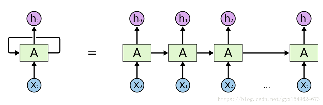
具体的，RNN网络会对前面信息进行记忆，并将其运用在当前输出的计算当中，即隐藏层的输入不仅包含输入层的输出还包含上一时刻隐藏层的输出。下图较为形象的显示了其工作方式：

二、LSTM神经网络

当遇到预测点与依赖点的相关信息距离比较远的时候就难以学到该相关信息，称为长时依赖问题。为很好解决这一问题，我们想到了LSTM神经网络，它是一种特殊的RNN。

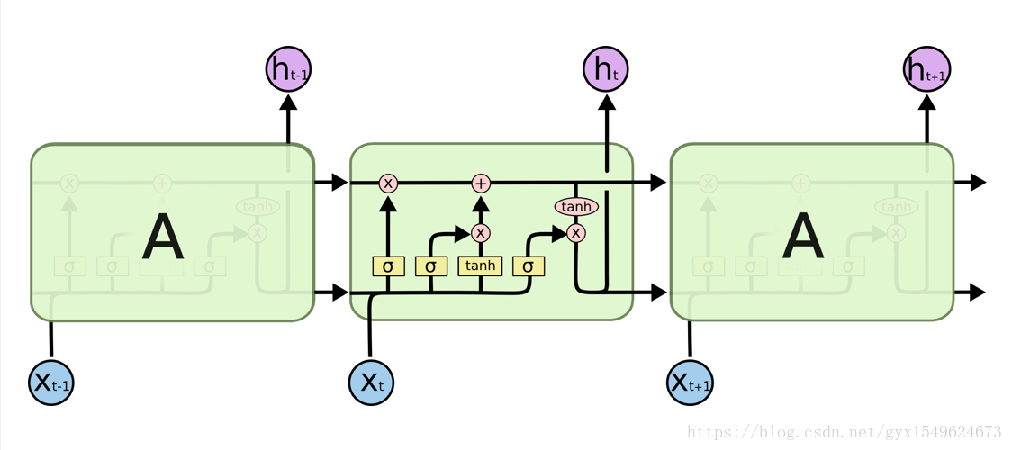
其模块结构图如下：

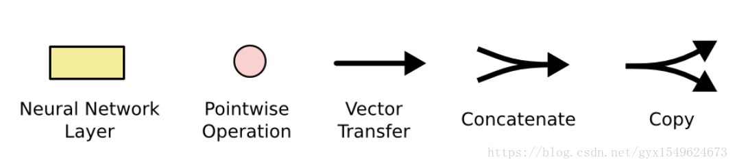
处理层各符号的表示的意思为：

LSTM通过一些“门”（输入门、遗忘门、输出门）结构让信息有选择性的影响网络中的每个时刻的状态。这里的所谓门就是sigmoid神经网络和一个按位做乘法的操作。叫做‘门’是因为sigmoid激活函数的全连接神经网络会输出0到1之间的数值，描述当前有多少信息量可以通过这个结构。

遗忘门的作用是让RNN忘记之前没有用的信息。输入们的作用就是根据当前结点输入xt，之前状态c(t-1)，上一时刻输出决定当前哪些信息进入到当前的ct。

三、代码样例

# 这里用mnist数据集来简单说明下lstm的搭建
import numpy as np
import tensorflow as tf
from tensorflow.examples.tutorials.mnist import input_data
# 首先观察下数据
mnist  = input_data.read_data_sets('MNIST_data/', one_hot=True)
print(mnist.train.images.shape)
# 使用LSTM来实现mnist的分类，将输入28*28的图像每一行看作输入像素序列，行行之间具有时间信息。即step=28
# 设置超参数
#超参数
lr = 0.001
training_inter = 100000
batch_size = 128
# display_step = 10 #

n_input = 28 # w
n_step = 28 # h
n_hidden = 128
n_classes = 10

# placeholder
x = tf.placeholder(tf.float32, [None, n_input, n_step])
y = tf.placeholder(tf.float32, [None, n_classes])

weights = {
    'in': tf.Variable(tf.random_normal([n_input, n_hidden])), # (28, 128)
    'out': tf.Variable(tf.random_normal([n_hidden, n_classes])) # (128, 10)
}
biases = {
    'in': tf.Variable(tf.constant(0.1, shape=[n_hidden])),
    'out': tf.Variable(tf.constant(0.1, shape=[n_classes]))
}

def RNN(x, weights, biases):
    # 原始的x是3维,需要将其变为2为的，才能和weight矩阵乘法
    # x=(128, 28, 28) ->> (128*28, 28)
    X = tf.reshape(x, [-1, n_input])
    X_in = tf.matmul(X, weights['in']) + biases['in'] # (128*28, 128)
    X_in = tf.reshape(X_in, [-1, n_step, n_hidden]) # (128, 28, 128)
    # 定义LSTMcell
    lstm_cell = tf.contrib.rnn.BasicLSTMCell(n_hidden)
    init_state = lstm_cell.zero_state(batch_size, dtype=tf.float32)
    outputs, final_state = tf.nn.dynamic_rnn(lstm_cell, X_in, initial_state=init_state, time_major=False)
    results = tf.matmul(final_state[1], weights['out']) + biases['out']
    return results

pre = RNN(x, weights, biases)
cost = tf.reduce_mean(tf.nn.softmax_cross_entropy_with_logits(labels=y, logits=pre))
train_op = tf.train.AdamOptimizer(lr).minimize(cost)

correct_pred = tf.equal(tf.argmax(pre, 1), tf.argmax(y, 1))
accuracy = tf.reduce_mean(tf.cast(correct_pred, tf.float32))

init = tf.global_variables_initializer()

with tf.Session() as sess:
    sess.run(init)
    step = 0
    while step*batch_size < training_inter:
        batch_xs, batch_ys = mnist.train.next_batch(batch_size)
        batch_xs = batch_xs.reshape([batch_size, n_step, n_input])
        sess.run([train_op], feed_dict={x: batch_xs, y: batch_ys})
        if step % 20 == 0:
            print(sess.run(accuracy, feed_dict={x: batch_xs, y: batch_ys}))
        step += 1

结果如下：

0.21875
0.6875
0.765625
0.828125
0.875
0.8515625
0.875
0.8671875
0.921875
0.890625
0.8671875
0.921875
0.9296875
0.921875
0.96875
0.9140625
0.96875
0.984375
0.9609375
0.9453125
0.9453125
0.953125
0.9609375
0.9453125
0.96875
0.9453125
0.9609375
0.9609375
0.96875
0.9609375
0.984375
0.9375
0.9609375
0.9609375
0.953125
0.9765625
0.9765625
0.9609375
0.9765625
0.9453125