ts(data = NA, start = 1, end = numeric(), frequency = 1,
deltat = 1, ts.eps = getOption(“ts.eps”), class = , names = )
start:第一次观测的时间。单个数字或两个整数的向量,它们指定一个自然时间单位和进入时间单位的(基于1的)样本数量
end:最后一次观测的时间,用与开始相同的方式指定
frequency:每单位时间的观测次数
deltat:连续观测之间采样周期的百分比;例如,月数据为1/12。
ts.eps:时间序列比较公差。如果频率的绝对差小于ts.eps,则认为频率相等
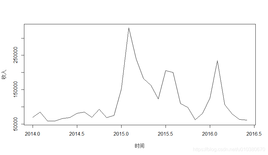
data2 <- read.csv("收入数据.csv")
head(data2)

data2.ts <- ts(data2[,2],frequency = 12,start = c(2014,1))
plot(data2.ts,xlab="时间",ylab="收入")
时间序列的平稳性检验
unitrootTest(x, lags = 1, type = c(“nc”, “c”, “ct”), title = NULL,
description = NULL)
lags:用于误差项校正的最大滞后数
type:描述单位根回归类型的字符串。正确的选项是“nc”表示没有截距(常数)或时间趋势的回归,“c”表示有截距(常数)但没有时间趋势的回归,“ct”表示有截距(常数)和时间趋势的回归。默认值是"c"
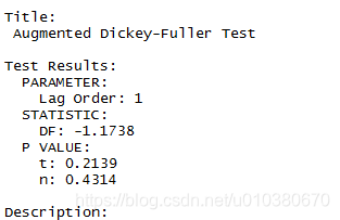
library(fUnitRoots)
unitrootTest(data2.ts)
测试返回一个类“fHTEST”的对象,该对象具有以下槽:
@call
the function call.函数调用
@data
a data frame with the input data.
@data.name
a character string giving the name of the data frame.
@test
a list object which holds the output of the underlying test function. 底层测试数据的输出
@title
a character string with the name of the test.
@description
a character string with a brief description of the test.
@test槽的条目包括以下组件:
$statistic
the value of the test statistic.
$parameter
the lag order. 滞后秩序
$p.value
the p-value of the test.
$method
a character string indicating what type of test was performed.指示执行什么类型的测试
$data.name
a character string giving the name of the data.
$alternative
a character string describing the alternative hypothesis. 描述替代假设
$name
the name of the underlying function, which may be wrapped.
$output
additional test results to be printed.
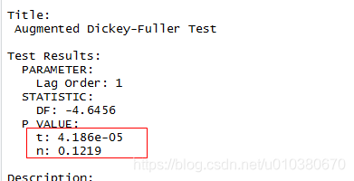
进行差分得到平稳序列
data2.ts.diff <- diff(data2.ts)
unitrootTest(data2.ts.diff)
data2.ts.decompose <- decompose(data2.ts)
plot(data2.ts.decompose)
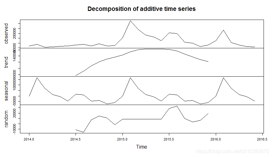
原始序列观测值、序列分解趋势图、序列分解季节变动图、序列分解噪声图
时间序列预测的主要方法:平均(平滑)预测法、长期趋势预测法、季节变动预测法、指数平滑预测法
指数平滑法是移动平均法中的一种,其特点在于给过去的观测值不一样的权重,即较近期观测值的权数比较远期观测值的权数要大。根据平滑次数不同,指数平滑法分为一次指数平滑法、二次指数平滑法和三次指数平滑法等。但它们的基本思想都是:预测值是以前观测值的加权和,且对不同的数据给予不同的权数,新数据给予较大的权数,旧数据给予较小的权数
HoltWinters(x, alpha = NULL, beta = NULL, gamma = NULL,
seasonal = c(“additive”, “multiplicative”),
start.periods = 2, l.start = NULL, b.start = NULL,
s.start = NULL,
optim.start = c(alpha = 0.3, beta = 0.1, gamma = 0.1),
optim.control = list())
alpha:霍尔特-温特斯滤波器的参数
beta:霍尔特-温特斯滤波器的贝塔参数。如果设置为FALSE,函数将进行指数平滑。
gamma:用于季节成分的伽马参数。如果设置为FALSE,则拟合非季节性模型
seasonal:选择“加法”(默认)或“乘法”季节性模型的字符串。前几个字符就足够了。(只在伽马非零时生效)
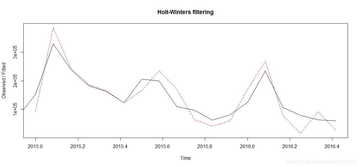
HoltWintersModel <- HoltWinters(data2.ts,alpha = TRUE,beta = TRUE,gamma = TRUE)
plot(HoltWintersModel,lty=1,lty.predicted=2)
HoltWintersForecast <- forecast(HoltWintersModel,h=6,)
acf(HoltWintersForecast$residuals,lag.max = 20,na.action = na.pass)
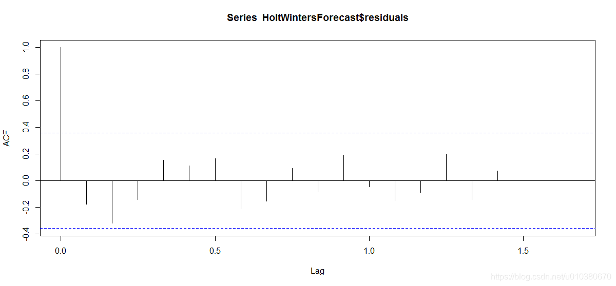
计算acf的最大延迟。默认为10*log10(N/m),其中N为观测次数,m为级数个数。将自动限制在比本系列观测值少一次的范围内。
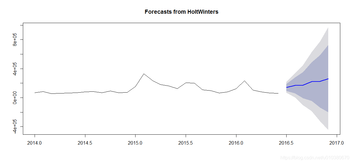
plot(HoltWintersForecast)
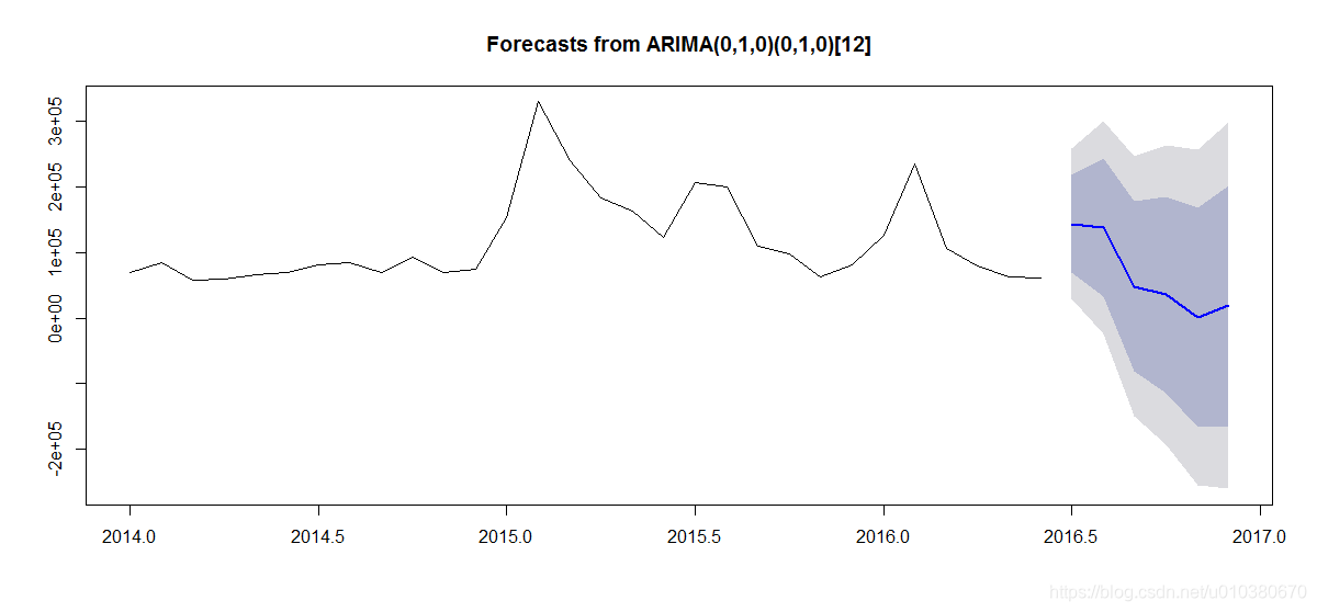
fit <- auto.arima(data2.ts)
fit.forecast <- forecast(fit,h=6)
plot(fit.forecast)