LSTM股票预测模型

1.LSTM简介

LSTM(Long Short-Term Memory)是长短期记忆网路，是一种时间递归神经网络，适合于处理和预测时间序列中间隔和延迟相对较长的重要事件。

LSTM已经在科技领域有了多种应用。基于LSTM的系统可以学习翻译语言、控制机器人、图像分析、文档摘要、语音识别、图像识别、手写识别、控制聊天机器人、预测疾病、点击率和股票、合成音乐等等任务。

------百度百科 https://baike.baidu.com/item/LSTM/17541102?fr=aladdin

2.LSTM工作原理

LSTM是RNN的特殊类型，因此我们先来介绍RNN的工作原理。

RNN(Recurrent Neural Network)是一类用于处理序列数据的神经网络。（时间序列数据是指在不同时间点上收集到的数据，这类数据反映了某一事物、现象等随时间的变化状态或程度。

神经网络包含了输入层、隐层、输出层，通过激活函数控制输出，层与层之间通过权值连接。激活函数是事先确定好的，那么神经网络模型通过训练“学”到的东西就蕴含在权值中。基础的神经网络只在层与层之间建立了权连接，RNN最大的不同之处就是在层之间的神经元之间也建立了权连接。如图：

X是输入，h是隐层单元，o是输出，L是损失函数，y是训练集的标签，U、V、W是权值

T时刻： ∅ 是激活函数

T时刻输出：

最终模型输出： σ 是激活函数

RNN的训练方法——BPTT

BPTT(back-propagation through time)算法是常用的训练RNN的方法，其实本质还是BP算法，只不过RNN是处理时间序列数据，所以要基于时间反向传播，故叫随时间反向传播。BPTT的中心思想和BP算法相同，沿着需要优化的参数的负梯度方向不断寻找更优的点直至收敛。

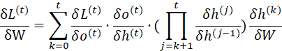
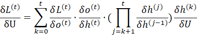
需要寻优的参数有三个，分别是U、V、W。与BP算法不同的是，其中W和U两个参数的寻优过程要追溯到之前的历史数据，参数V相对简单只须关注目前。

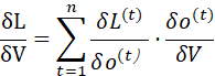
参数V的偏导数：

RNN的损失函数是随时间累加的，所以不能只求t时刻的偏导

LSTM是RNN的一种变体，RNN由于梯度消失的原因只能有短期记忆，LSTM网络通过精妙的门控制将短期记忆与长期记忆结合起来，并且一定程度上解决了梯度消失的问题。

所有的RNN都具有一种重复神经网络模块的链式形式。在标准RNN中，这个重复的结构模块只有一个非常简单的结构，例如一个tanh层。

LSTM 同样是这样的结构，但是重复的模块拥有一个不同的结构。不同于单一神经网络

层，这里是有四个，以一种非常特殊的方式进行交互。

黄色的矩形是学习得到的神经网络层粉色的圆形表示一些运算操作，诸如加法乘法
黑色的单箭头表示向量的传输
两个箭头合成一个表示向量的连接
一个箭头分开表示向量的复制

3.LSTM核心思想

LSTM的关键在于细胞的状态整个(绿色的图表示的是一个cell)，和穿过细胞的那条水平线。细胞状态类似于传送带。直接在整个链上运行，只有一些少量的线性交互。信息在上面流传保持不变会很容易。

若只有上面的那条水平线是没办法实现添加或者删除信息的。而是通过一种叫做门（gates）的结构来实现的。

门可以实现选择性地让信息通过，主要是通过一个 sigmoid 的神经层和一个逐点相乘的操作来实现的。

sigmoid 层输出（是一个向量）的每个元素都是一个在 0 和 1 之间的实数，表示让对应信息通过的权重（或者占比）。比如， 0 表示“不让任何信息通过”， 1 表示“让所有信息通过”。

LSTM通过三个这样的本结构来实现信息的保护和控制。这三个门分别输入门、遗忘门和输出门。

遗忘门：

作用对象：细胞状态

作用：使细胞状态中的信息选择性遗忘

输入门：

作用对象：细胞状态

作用：将新的信息选择性的记录到细胞状态中

输出门

作用对象：隐层ht

利用LSTM进行股票预测的代码：

输入：

Date:日期

Time:具体时刻

High:最高价

Low:最低价

Close:收盘价

Adj Close:已调整的收盘价

Volume:交易量

Label:下一时刻最高价

import pandas as pd
import numpy as np
import matplotlib.pyplot as plt
import tensorflow as tf

rnn_unit=10 #隐层神经元的个数
lstm_layers=2 #隐层层数
input_size=6
output_size=1
lr=0.0006 #学习率
#——————————导入数据———---------
f=open('SH000001.csv')
df=pd.read_csv(f) #读入股票数据
data=df.iloc[:,2:9].values #取第3-10列
data[:1]

def get_train_data(batch_size=60,time_step=20,train_begin=0,train_end=5800):
batch_index=[]
data_train=data[train_begin:train_end]
normalized_train_data=(data_train-np.mean(data_train,axis=0))/np.std(data_train,axis=0) #标准化
train_x,train_y=[],[] #训练集
for i in range(len(normalized_train_data)-time_step):
if i % batch_size==0:
batch_index.append(i)
x=normalized_train_data[i:i+time_step,:6]
y=normalized_train_data[i:i+time_step,6,np.newaxis]
train_x.append(x.tolist())
train_y.append(y.tolist())
batch_index.append((len(normalized_train_data)-time_step))
return batch_index,train_x,train_y

#获取测试集
def get_test_data(time_step=20,test_begin=5800):
data_test=data[test_begin:9800]
mean=np.mean(data_test,axis=0)
std=np.std(data_test,axis=0)
normalized_test_data=(data_test-mean)/std #标准化
size=(len(normalized_test_data)+time_step-1)//time_step #有size个sample
test_x,test_y=[],[]
for i in range(size-1):
x=normalized_test_data[i*time_step:(i+1)*time_step,:6]
y=normalized_test_data[i*time_step:(i+1)*time_step,6]
test_x.append(x.tolist())
test_y.extend(y)
test_x.append((normalized_test_data[(i+1)*time_step:,:6]).tolist())
test_y.extend((normalized_test_data[(i+1)*time_step:,6]).tolist())
return mean,std,test_x,test_y

#——————————定义神经网络变量————————————
#输入层、输出层权重、偏置、dropout参数

weights={
'in':tf.Variable(tf.random_normal([input_size,rnn_unit])),
'out':tf.Variable(tf.random_normal([rnn_unit,1]))
}
biases={
'in':tf.Variable(tf.constant(0.1,shape=[rnn_unit,])),
'out':tf.Variable(tf.constant(0.1,shape=[1,]))
}
keep_prob = tf.placeholder(tf.float32, name='keep_prob')

#—————————定义神经网络变量————————————
def lstmCell():
#basicLstm单元
basicLstm = tf.nn.rnn_cell.BasicLSTMCell(rnn_unit)
# dropout
drop = tf.nn.rnn_cell.DropoutWrapper(basicLstm, output_keep_prob=keep_prob)
return basicLstm

def lstm(X):

batch_size=tf.shape(X)[0]
time_step=tf.shape(X)[1]
w_in=weights['in']
b_in=biases['in']
input=tf.reshape(X,[-1,input_size]) #需要将tensor转成2维进行计算，计算后的结果作为隐藏层的输入
input_rnn=tf.matmul(input,w_in)+b_in
input_rnn=tf.reshape(input_rnn,[-1,time_step,rnn_unit]) #将tensor转成3维，作为lstm cell的输入
cell = tf.nn.rnn_cell.MultiRNNCell([lstmCell() for i in range(lstm_layers)])
init_state=cell.zero_state(batch_size,dtype=tf.float32)
output_rnn,final_states=tf.nn.dynamic_rnn(cell, input_rnn,initial_state=init_state, dtype=tf.float32)
output=tf.reshape(output_rnn,[-1,rnn_unit])
w_out=weights['out']
b_out=biases['out']
pred=tf.matmul(output,w_out)+b_out
return pred,final_states

#————————————————预测模型————————————————————
def prediction(time_step=20):
X=tf.placeholder(tf.float32, shape=[None,time_step,input_size])
mean,std,test_x,test_y=get_test_data(time_step)
with tf.variable_scope("sec_lstm",reuse=tf.AUTO_REUSE):#reuse=tf.AUTO_REUSE
pred,_=lstm(X)
saver=tf.train.Saver(tf.global_variables())
with tf.Session() as sess:
#参数恢复
module_file = tf.train.latest_checkpoint('model_save2')
saver.restore(sess, module_file)
test_predict=[]
for step in range(len(test_x)-1):
prob=sess.run(pred,feed_dict={X:[test_x[step]],keep_prob:1})
predict=prob.reshape((-1))
test_predict.extend(predict)
test_y=np.array(test_y)*std[6]+mean[6]
test_predict=np.array(test_predict)*std[6]+mean[6]
acc=np.average(np.abs(test_predict-test_y[:len(test_predict)])/test_y[:len(test_predict)]) #偏差程度
print("The accuracy of this predict:",acc)
#以折线图表示结果
plt.figure()
plt.plot(list(range(len(test_predict))), test_predict, color='b',)
plt.plot(list(range(len(test_y))), test_y, color='r')
plt.show()

prediction()

猜你喜欢