Python基于LSTM预测特斯拉股票

Python基于LSTM预测特斯拉股票

提示：前言
Python基于LSTM预测特斯拉股票

股票预测是指：对股市具有深刻了解的证券分析人员根据股票行情的发展进行的对未来股市发展方向以及涨跌程度的预测行为。这种预测行为只是基于假定的因素为既定的前提条件为基础的。

LSTM的全称是Long Short Term Memory，顾名思义，它具有记忆长短期信息的能力的神经网络。LSTM首先在1997年由Hochreiter & Schmidhuber [1] 提出，由于深度学习在2012年的兴起，LSTM又经过了若干代大牛(Felix Gers, Fred Cummins, Santiago Fernandez, Justin Bayer, Daan Wierstra, Julian Togelius, Faustino Gomez, Matteo Gagliolo, and Alex Gloves)的发展，由此便形成了比较系统且完整的LSTM框架，并且在很多领域得到了广泛的应用。本文着重介绍深度学习时代的LSTM。

---

提示：写完文章后，目录可以自动生成，如何生成可参考右边的帮助文档

---

前言

---

提示：以下是本篇文章正文内容，下面案例可供参考

一、导入包

import pandas as pd
import numpy as np

import matplotlib.pyplot as plt
import seaborn as sns
sns.set_style('whitegrid')
plt.style.use("fivethirtyeight")
%matplotlib inline
              
from datetime import datetime

二、下载数据

下载特斯拉股票

df=pd.read_csv("/tesla-inc-tsla-stock-price/TSLA.csv")
TESLA=df

company_list = [TESLA]
company_name = ["TESLA"]

for company, com_name in zip(company_list, company_name):
    company["company_name"] = com_name
    
df = pd.concat(company_list, axis=0)
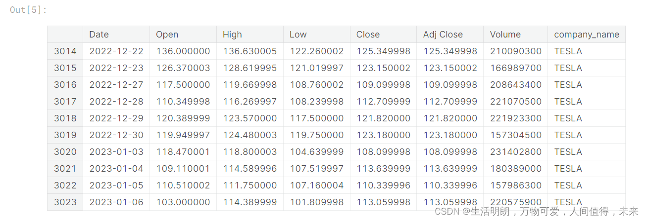
df.tail(10)

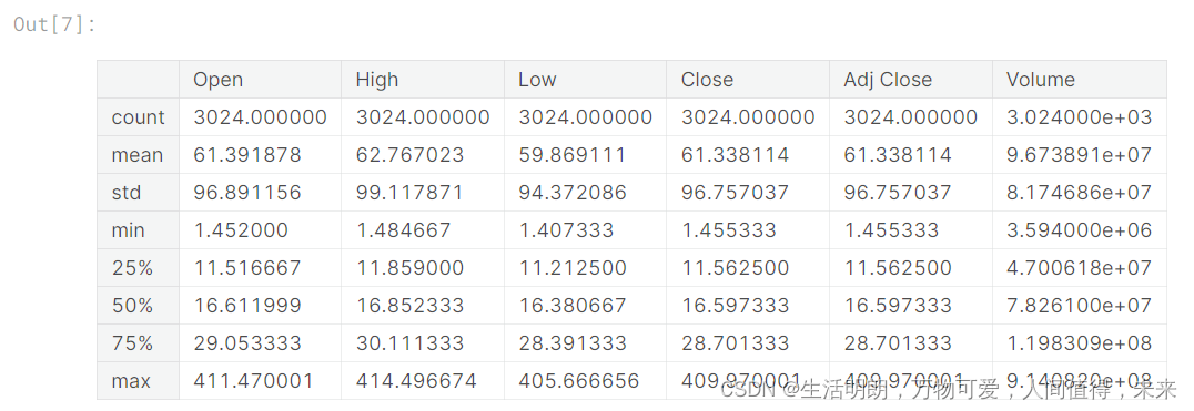
描述性统计

df.describe()

df.info()

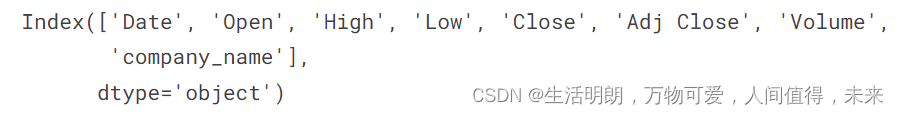
df.columns

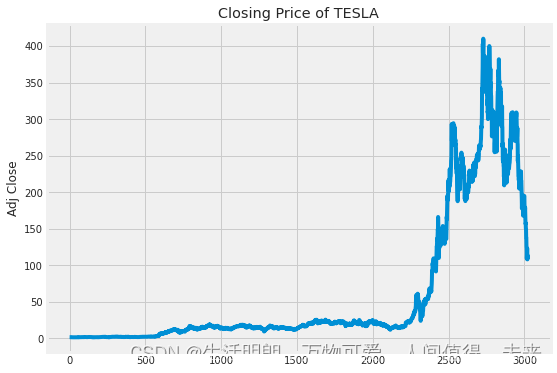
股票价格走势图

plt.figure(figsize=(15, 10))
plt.subplots_adjust(top=1.25, bottom=1.2)

for i, company in enumerate(company_list, 1):
    plt.subplot(2, 2, i)
    company['Adj Close'].plot()
    plt.ylabel('Adj Close')
    plt.xlabel(None)
    plt.title("Closing Price of TESLA")
  
    
plt.tight_layout()

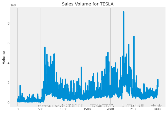
成交量走势图

# Now let's plot the total volume of stock being traded each day
plt.figure(figsize=(15, 10))
plt.subplots_adjust(top=1.25, bottom=1.2)

for i, company in enumerate(company_list, 1):
    plt.subplot(2, 2, i)
    company['Volume'].plot()
    plt.ylabel('Volume')
    plt.xlabel(None)
    plt.title("Sales Volume for TESLA")
    
plt.tight_layout()

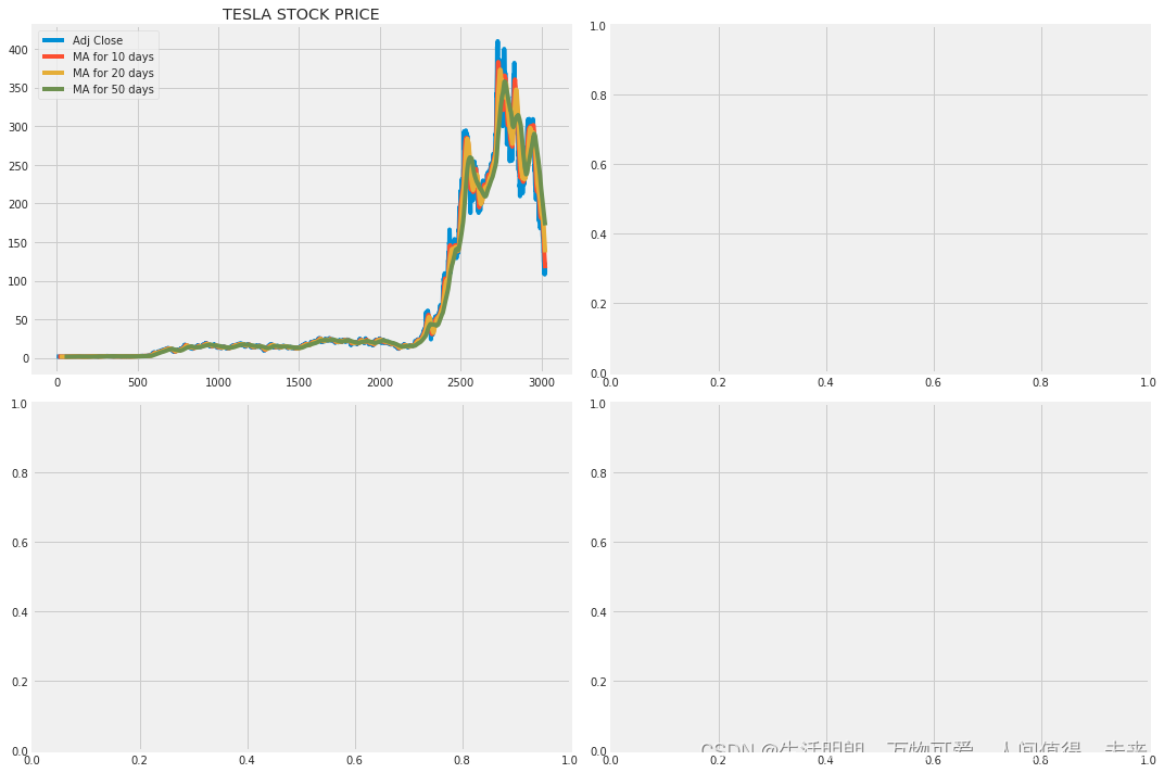
三、构造技术指标

ma_day = [10, 20, 50]

for ma in ma_day:
    for company in company_list:
        column_name = f"MA for {
      
      ma} days"
        company[column_name] = company['Adj Close'].rolling(ma).mean()
        

fig, axes = plt.subplots(nrows=2, ncols=2)
fig.set_figheight(10)
fig.set_figwidth(15)

TESLA[['Adj Close', 'MA for 10 days', 'MA for 20 days', 'MA for 50 days']].plot(ax=axes[0,0])
axes[0,0].set_title('TESLA STOCK PRICE')
fig.tight_layout()

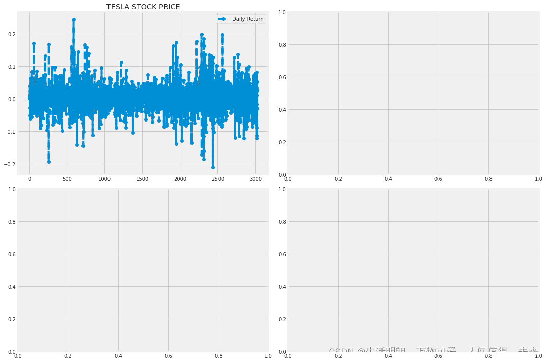
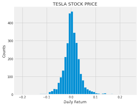
收益率图

# We'll use pct_change to find the percent change for each day
for company in company_list:
    company['Daily Return'] = company['Adj Close'].pct_change()

# Then we'll plot the daily return percentage
fig, axes = plt.subplots(nrows=2, ncols=2)
fig.set_figheight(10)
fig.set_figwidth(15)

TESLA['Daily Return'].plot(ax=axes[0,0], legend=True, linestyle='--', marker='o')
axes[0,0].set_title('TESLA STOCK PRICE')
fig.tight_layout()

plt.figure(figsize=(12, 9))

for i, company in enumerate(company_list, 1):
    plt.subplot(2, 2, i)
    company['Daily Return'].hist(bins=50)
    plt.xlabel('Daily Return')
    plt.ylabel('Counts')
    plt.title("TESLA STOCK PRICE")
    
plt.tight_layout()

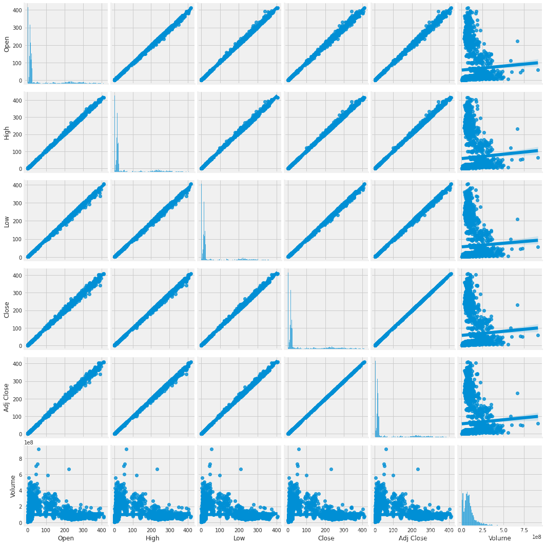
# We can simply call pairplot on our DataFrame for an automatic visual analysis 
# of all the comparisons

sns.pairplot(df, kind='reg')

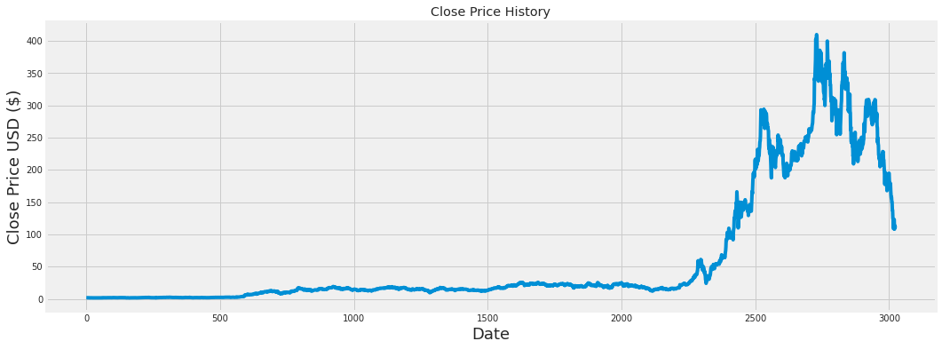
plt.figure(figsize=(16,6))
plt.title('Close Price History')
plt.plot(df['Close'])
plt.xlabel('Date', fontsize=18)
plt.ylabel('Close Price USD ($)', fontsize=18)
plt.show()

# Create a new dataframe with only the 'Close column 
data = df.filter(['Close'])
# Convert the dataframe to a numpy array
dataset = data.values
# Get the number of rows to train the model on
training_data_len = int(np.ceil( len(dataset) * .95 ))

training_data_len

四、数据标准化

使⽤sklearn进⾏对数据标准化、归⼀化以及将数据还原的⽅法
在对模型训练时，为了让模型尽快收敛，⼀件常做的事情就是对数据进⾏预处理。
这⾥通过使⽤sklearn.preprocess模块进⾏处理。
⼀、标准化和归⼀化的区别
归⼀化其实就是标准化的⼀种方式，只不过归⼀化是将数据映射到了[0,1]这个区间中。
标准化则是将数据按照比例缩放，使之放到⼀个特定区间中。标准化后的数据的均值＝0，标准差＝1，因而标准化的数据可正可负。

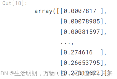
# Scale the data
from sklearn.preprocessing import MinMaxScaler

scaler = MinMaxScaler(feature_range=(0,1))
scaled_data = scaler.fit_transform(dataset)

scaled_data

五、划分训练集和测试集

训练集

# Create the training data set 
# Create the scaled training data set
train_data = scaled_data[0:int(training_data_len), :]
# Split the data into x_train and y_train data sets
x_train = []
y_train = []

for i in range(60, len(train_data)):
    x_train.append(train_data[i-60:i, 0])
    y_train.append(train_data[i, 0])
    if i<= 61:
        print(x_train)
        print(y_train)
        print()
        
# Convert the x_train and y_train to numpy arrays 
x_train, y_train = np.array(x_train), np.array(y_train)

# Reshape the data
x_train = np.reshape(x_train, (x_train.shape[0], x_train.shape[1], 1))
# x_train.shape

测试集

# Create the testing data set
# Create a new array containing scaled values from index 1543 to 2002 
test_data = scaled_data[training_data_len - 60: , :]
# Create the data sets x_test and y_test
x_test = []
y_test = dataset[training_data_len:, :]
for i in range(60, len(test_data)):
    x_test.append(test_data[i-60:i, 0])
    
# Convert the data to a numpy array
x_test = np.array(x_test)

# Reshape the data
x_test = np.reshape(x_test, (x_test.shape[0], x_test.shape[1], 1 ))

六、建立LSTM模型并训练模型

from keras.models import Sequential
from keras.layers import Dense, LSTM

# Build the LSTM model
model = Sequential()
model.add(LSTM(128, return_sequences=True, input_shape= (x_train.shape[1], 1)))
model.add(LSTM(64, return_sequences=False))
model.add(Dense(25))
model.add(Dense(1))

# Compile the model
model.compile(optimizer='adam', loss='mean_squared_error')

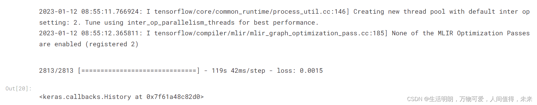
# Train the model
model.fit(x_train, y_train, batch_size=1, epochs=1)

七、预测

# Get the models predicted price values 
predictions = model.predict(x_test)
predictions = scaler.inverse_transform(predictions)

# Get the root mean squared error (RMSE)
rmse = np.sqrt(np.mean(((predictions - y_test) ** 2)))
rmse

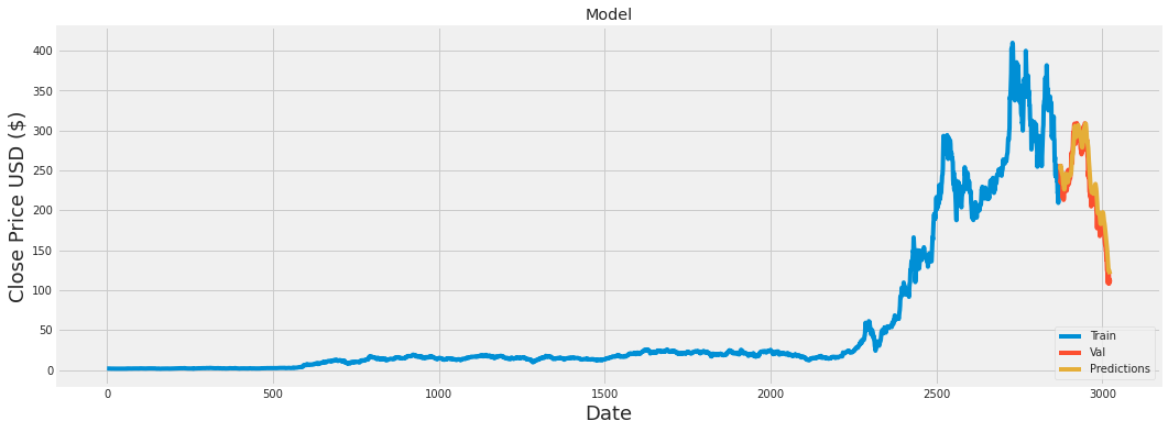
打印预测结果

# Plot the data
train = data[:training_data_len]
valid = data[training_data_len:]
valid['Predictions'] = predictions
# Visualize the data
plt.figure(figsize=(16,6))
plt.title('Model')
plt.xlabel('Date', fontsize=18)
plt.ylabel('Close Price USD ($)', fontsize=18)
plt.plot(train['Close'])
plt.plot(valid[['Close', 'Predictions']])
plt.legend(['Train', 'Val', 'Predictions'], loc='lower right')
plt.show()