比赛相关部分练习总结
df_train = pd.read_csv('C:/Users/zhangy/Desktop/kaggle_competition_feature_engineering/kaggle_bike_competition_train.csv')
# print(train.shape)
# print(train.apply(lambda x:sum(x.isnull())))              #查看每一列缺失值的数量
df_train['month'] = pd.DatetimeIndex(df_train.datetime).month
df_train['day'] = pd.DatetimeIndex(df_train.datetime).dayofweek
df_train['hour'] = pd.DatetimeIndex(df_train.datetime).hour

df_train_origin = df_train
df_train=df_train.drop(['datetime'],axis=1)
df_train_target = df_train['count']                 #训练集标签
df_train_data = df_train.drop(['count'],axis=1)     #训练集数据

X_train,X_test,y_train,y_test=train_test_split(df_train_data,df_train_target,test_size=0.2,random_state=0)
# clf = RandomForestRegressor(n_estimators=100)
# clf.fit(X_train,y_train)
# print(clf.score(X_train,y_train))
# print(clf.score(X_test,y_test))
RandomForest:
sklearn.ensemble.RandomForestRegressor(  n_estimators=10,
                                             criterion='mse',
                                             max_depth=None,
                                             min_samples_split=2,
                                             min_samples_leaf=1,
                                             min_weight_fraction_leaf=0.0,
                                             max_features='auto',
                                             max_leaf_nodes=None,
                                             min_impurity_split=1e-07,
                                             bootstrap=True,
                                             oob_score=False,
                                             n_jobs=1,
                                             random_state=None,
                                             verbose=0,
                                             warm_start=False)
其中关于决策树的参数:
criterion: “mse”来选择最合适的节点。
splitter: ”best” or “random”(default=”best”)随机选择属性还是选择不纯度最大的属性,建议用默认。
max_features: 选择最适属性时划分的特征不能超过此值。
当为整数时,即最大特征数;当为小数时,训练集特征数*小数;
if “auto”, then max_features=sqrt(n_features).
If “sqrt”, thenmax_features=sqrt(n_features).
If “log2”, thenmax_features=log2(n_features).
If None, then max_features=n_features.
max_depth: (default=None)设置树的最大深度,默认为None,这样建树时,会使每一个叶节点只有一个类别,或是达到min_samples_split。
min_samples_split: 根据属性划分节点时,每个划分最少的样本数。
min_samples_leaf: 叶子节点最少的样本数。
max_leaf_nodes: (default=None)叶子树的最大样本数。
min_weight_fraction_leaf: (default=0) 叶子节点所需要的最小权值
verbose: (default=0) 是否显示任务进程
关于随机森林特有的参数:
n_estimators=10: 决策树的个数,越多越好,但是性能就会越差,至少100左右(具体数字忘记从哪里来的了)可以达到可接受的性能和误差率。
bootstrap=True: 是否有放回的采样。
oob_score=False: oob(out of band,带外)数据,即:在某次决策树训练中没有被bootstrap选中的数据。多单个模型的参数训练,我们知道可以用cross validation(cv)来进行,但是特别消耗时间,而且对于随机森林这种情况也没有大的必要,所以就用这个数据对决策树模型进行验证,算是一个简单的交叉验证。性能消耗小,但是效果不错。
n_jobs=1: 并行job个数。这个在ensemble算法中非常重要,尤其是bagging(而非boosting,因为boosting的每次迭代之间有影响,所以很难进行并行化),因为可以并行从而提高性能。1=不并行;n:n个并行;-1:CPU有多少core,就启动多少job
warm_start=False: 热启动,决定是否使用上次调用该类的结果然后增加新的。
class_weight=None: 各个label的权重。
进行预测可以有几种形式:
predict_proba(x): 给出带有概率值的结果。每个点在所有label的概率和为1.
predict(x): 直接给出预测结果。内部还是调用的predict_proba(),根据概率的结果看哪个类型的预测值最高就是哪个类型。
predict_log_proba(x): 和predict_proba基本上一样,只是把结果给做了log()处理。
# clf = svm.SVC(kernel='rbf',C=10,gamma=0.001,probability=True)
# clf.fit(X_train,y_train)
#
# print(clf.score(X_train,y_train))
# print(clf.score(X_test,y_test))
SVM:
sklearn.svm.SVC(C=1.0, kernel=‘rbf’, degree=3, gamma=‘auto’, coef0=0.0, shrinking=True, probability=False,
tol=0.001, cache_size=200, class_weight=None, verbose=False, max_iter=-1, decision_function_shape=None,random_state=None)
参数:
l C:C-SVC的惩罚参数C?默认值是1.0
C越大,相当于惩罚松弛变量,希望松弛变量接近0,即对误分类的惩罚增大,趋向于对训练集全分对的情况,这样对训练集测试时准确率很高,但泛化能力弱。C值小,对误分类的惩罚减小,允许容错,将他们当成噪声点,泛化能力较强。
l kernel :核函数,默认是rbf,可以是‘linear’, ‘poly’, ‘rbf’, ‘sigmoid’, ‘precomputed’
0 – 线性:u’v
1 – 多项式:(gamma*u’*v + coef0)^degree
2 – RBF函数:exp(-gamma|u-v|^2)
3 –sigmoid:tanh(gamma*u’*v + coef0)
l degree :多项式poly函数的维度,默认是3,选择其他核函数时会被忽略。
l gamma : ‘rbf’,‘poly’ 和‘sigmoid’的核函数参数。默认是’auto’,则会选择1/n_features
l coef0 :核函数的常数项。对于‘poly’和 ‘sigmoid’有用。
l probability :是否采用概率估计?.默认为False
l shrinking :是否采用shrinking heuristic方法,默认为true
l tol :停止训练的误差值大小,默认为1e-3
l cache_size :核函数cache缓存大小,默认为200
l class_weight :类别的权重,字典形式传递。设置第几类的参数C为weight*C(C-SVC中的C)
l verbose :允许冗余输出?
l max_iter :最大迭代次数。-1为无限制。
l decision_function_shape :‘ovo’, ‘ovr’ or None, default=None3
l random_state :数据洗牌时的种子值,int值
主要调节的参数有:C、kernel、degree、gamma、coef0
tuned_parameters = [{'n_estimators':[10,100,500]}]
scores = ['r2']
for score in scores:
    clf = GridSearchCV(RandomForestRegressor(),tuned_parameters,cv=5,scoring=score)
    clf.fit(X_train,y_train)
    print("最佳参数为:")
    print(clf.best_params_)
    print("得分分别为:")
    for params, mean_score, scores in clf.grid_scores_:
        print("%0.3f (+/-%0.03f) for %r"% (mean_score, scores.std()/2, params))
GridSearchCV:
sklearn.model_selection.GridSearchCV(estimator, param_grid, scoring=None, fit_params=None, n_jobs=1, iid=True, refit=True, cv=None, verbose=0, pre_dispatch=‘2*n_jobs’, error_score=’raise’, return_train_score=’warn’)

estimator —— 模型
param_grid —— dict or list of dictionaries
scoring ---- 评分函数
fit_params --- dict, optional
n_jobs ------并行任务个数,int, default=1
pre_dispatch ------ int, or string, optional ‘2*n_jobs’
iid ----- boolean, default=True
cv ----- int, 交叉验证,默认3
refit ---- boolean, or string, default=True
verbose ----- integer
error_score ------ ‘raise’ (default) or numeric
总结一些特征查看处理小技巧
print(train.apply(lambda x:sum(x.isnull()))) #查看每列特征缺失值个数
print(train['grade'].value_counts()) #查看某列数据不同值的个数
print(train['int_rate'].unique()) #查看某特征中只有一个值得项
train.drop(['id','member_id'],axis=1,inplace=True) #删掉数据集中的某些列
train.boxplot(column=['open_acc'],return_type='axes') #绘制某一列特征的箱体图
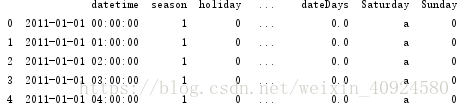
temp = pd.DatetimeIndex(train['datetime'])
train['date'] = temp.date
train['time'] = temp.time #2011/1/1 2:00:00原特征,现在讲时间和日期分开
train['hour'] = pd.to_datetime(train.time, format="%H:%M:%S")
train['hour'] = pd.Index(train['hour']).hour #再单独把hour拿出来
train['dayofweek'] = pd.DatetimeIndex(train.date).dayofweek #把数据转换为周几
train['dateDays'] = (train.date - train.date[0]).astype('timedelta64[D]') #表示距离第一套的时长
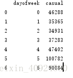
byday = train.groupby('dayofweek')
print(byday['casual'].sum().reset_index()) #统计一周每天‘casual’特征的情况
train['Saturday']=0
train.Saturday[train.dayofweek==5]='a'
train['Sunday']=0
train.Sunday[train.dayofweek==6]='b' #单独去除某一天作为特征,并赋值(任意)
train['Saturday']=0
train.Saturday[train.dayofweek==5]='a'

train['Sunday']=0
train.Sunday[train.dayofweek==6]='b'				#单独去除某一天作为特征,并赋值(任意)
dataRel = train.drop(['datetime', 'count','date','time','dayofweek'], axis=1) #删除某些列
对于pandas的dataframe我们有方法/函数可以直接转成python中的dict。另外,在这里我们要对离散值和连续值特征区分一下了,以便之后分开做不同的特征处理
featureConCols = ['temp','atemp','humidity','windspeed','dateDays','hour']
dataFeatureCon = dataRel[featureConCols]
dataFeatureCon = dataFeatureCon.fillna( 'NA' ) #in case I missed any
X_dictCon = dataFeatureCon.T.to_dict().values()
把离散值的属性放到另外一个dict中
featureCatCols = ['season','holiday','workingday','weather','Saturday', 'Sunday']
dataFeatureCat = dataRel[featureCatCols]
dataFeatureCat = dataFeatureCat.fillna( 'NA' ) #in case I missed any
X_dictCat = dataFeatureCat.T.to_dict().values()
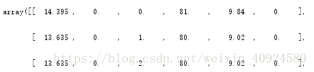
向量化特征
vec = DictVectorizer(sparse = False)
X_vec_con = vec.fit_transform(X_dictCon)
X_vec_cat = vec.fit_transform(X_dictCat)
对连续值属性做一些处理,最基本的当然是标准化,让连续值属性处理过后均值为0,方差为1。
from sklearn import preprocessing
# 标准化连续值数据
scaler = preprocessing.StandardScaler().fit(X_vec_con)
X_vec_con = scaler.transform(X_vec_con)				#标准化连续值向量

类别特征编码,最常用的当然是one-hot编码咯,比如颜色 红、蓝、黄 会被编码为[1, 0, 0],[0, 1, 0],[0, 0, 1]
from sklearn import preprocessing
# one-hot编码
enc = preprocessing.OneHotEncoder()
enc.fit(X_vec_cat)
X_vec_cat = enc.transform(X_vec_cat).toarray()

from sklearn.preprocessing import LabelEncoder
le = LabelEncoder()
y = le.fit_transform(y) # 把字符串标签转换为整数,恶性-1,良性-0	标签编码

k-fold交叉验证:
1自己手写!!
from sklearn.cross_validation import StratifiedKFold
import numpy as np

scores = []
kfold = StratifiedKFold(y=y_train, n_folds=10, random_state=1) # n_folds参数设置为10份
for train_index, test_index in kfold:
    pipe_lr.fit(X_train[train_index], y_train[train_index])
    score = clf.score(X_train[test_index], y_train[test_index])
    scores.append(score)
    print('类别分布: %s, 准确度: %.3f' % (np.bincount(y_train[train_index]), score))

2、sklearn
from sklearn.cross_validation import cross_val_score
scores = cross_val_score(estimator=clf, X=X_train, y=y_train, cv=10, n_jobs=1)
F-score:
from sklearn.metrics import confusion_matrix
clf.fit(X_train, y_train)
y_pred = clf.predict(X_test)
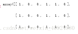
confmat = confusion_matrix(y_true=y_test, y_pred=y_pred)
confmat即为:
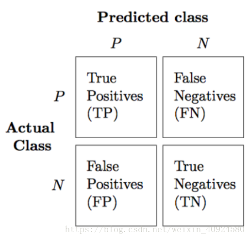
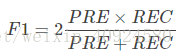
在类别很不平衡的机器学习系统中,我们通常用precision(PRE)和recall(REC)来度量模型的性能,下面我给出它们的公式:
在实际中,我们通常结合两者,组成F1-score:

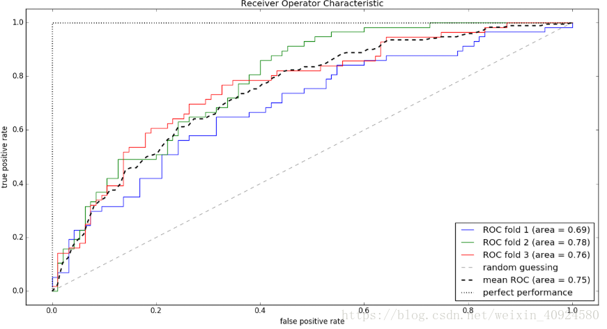
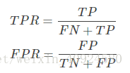
在介绍ROC曲线前,我先给出true positive rate(TPR)和false positive rate(FPR)的定义:
from sklearn.metrics import roc_curve, auc
from scipy import interp

X_train2 = X_train[:, [4, 14]]
cv = StratifiedKFold(y_train, n_folds=3, random_state=1)
fig = plt.figure()

mean_tpr = 0.0
mean_fpr = np.linspace(0, 1, 100)
all_tpr = []

# plot每个fold的ROC曲线,这里fold的数量为3,被StratifiedKFold指定
for i, (train, test) in enumerate(cv):
    # 返回预测的每个类别(这里为0或1)的概率
    probas = pipe_lr.fit(X_train2[train], y_train[train]).predict_proba(X_train2[test])
    fpr, tpr, thresholds = roc_curve(y_train[test], probas[:, 1], pos_label=1)
    mean_tpr += interp(mean_fpr, fpr, tpr)
    mean_tpr[0] = 0.0
    roc_auc = auc(fpr, tpr)
    plt.plot(fpr, tpr, linewidth=1, label='ROC fold %d (area = %0.2f)' % (i+1, roc_auc))


# plot random guessing line
plt.plot([0, 1], [0, 1], linestyle='--', color=(0.6, 0.6, 0.6), label='random guessing')

mean_tpr /= len(cv)
mean_tpr[-1] = 1.0
mean_auc = auc(mean_fpr, mean_tpr)
plt.plot(mean_fpr, mean_tpr, 'k--', label='mean ROC (area = %0.2f)' % mean_auc, lw=2)
# plot perfect performance line
plt.plot([0, 0, 1], [0, 1, 1], lw=2, linestyle=':', color='black', label='perfect performance')
# 设置x,y坐标范围
plt.xlim([-0.05, 1.05])
plt.ylim([-0.05, 1.05])
plt.xlabel('false positive rate')
plt.ylabel('true positive rate')
plt.title('Receiver Operator Characteristic')
plt.legend(loc="lower right")
plt.show()
roc官方文档:
http://scikit-learn.org/stable/modules/generated/sklearn.metrics.roc_curve.html