MXNet动手学深度学习-线性回归

线性回归

线性回归输出是⼀个连 续值，因此适⽤于回归问题。回归问题在实际中很常⻅，例如预测房屋价格、⽓温、销售额等连续值的问题。

本节中将会实现房屋价格预测这一实例。

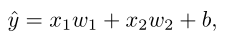
设房屋的⾯积为 $x_1$，房龄为 $x_2$ ，售出价格为 $y$。我们需要建⽴基于输⼊ $x_1$和 $x_2$ 来计算输出 $y$的表达式，也就是模型（model）。顾名思义，线性回归假设输出与各个输⼊之间是线性关系：

# 代码

#线性回归的从零开始实现
from IPython import display
from matplotlib import pyplot as plt
from mxnet import autograd, nd
import random

# 生成数据集
num_inputs = 2
num_examples = 1000
true_w = [2, -3.4]
true_b = 4.2

features = nd.random.normal(scale = 1, shape = (num_examples, num_inputs))
labels = true_w[0] * features[:, 0] + true_w[1] * features[:, 1] + true_b
labels = nd.random.normal(scale = 0.01, shape = labels.shape)
#print(features[0:10]) #测试使用
#print(labels[0:10]) #测试使用

# 定义函数data_iter，函数的作用：每次返回batch_size个随机样本的features和labels
def data_iter(batch_size, features, labels):
    num_examples = len(features)
    #print(num_examples)
    indices = list(range(num_examples))
    #print(indices)
    random.shuffle(indices) #将indices打乱
    #print(indices)
    for i in range(0, num_examples, batch_size):
        j = nd.array(indices[i:min(i + batch_size, num_examples)])
        yield features.take(j), labels.take(j)



batch_size = 10
for X, y in data_iter(batch_size, features, labels):
    print(X, y)
    break

w = nd.random.normal(scale = 0.01, shape = (num_inputs, 1))
b = nd.zeros(shape = (1,))

w.attach_grad()
b.attach_grad()
def linreg(X, w, b):
    return nd.dot(X, w) + b

def squared_loss(y_hat, y):
    return (y_hat - y.reshape(y_hat.shape)) ** 2 / 2

def sgd(params, lr, batch_size):
    for param in params:
        param[:] = param - lr * param.grad / batch_size

lr = 0.03
num_epochs = 3
net = linreg
loss = squared_loss

for epoch in range(num_epochs):
    for X, y in data_iter(batch_size, features, labels):
        with autograd.record():
            l = loss(net(X, w, b), y)
        l.backward()
        sgd([w, b], lr, batch_size)
    train_l = loss(net(features, w, b), labels)
    print('epoch %d, loss %f' % (epoch + 1, train_l.mean().asnumpy()))

运行结果

epoch 1, loss 0.000051
epoch 2, loss 0.000050
epoch 3, loss 0.000050

总结

在这个练习中，第一步首先生成了数据集，并没有使用真实的数据集进行实验。然后，读取数据，初始化模型参数，定义模型，定义损失函数、定义优化函数、最后进行模型的训练。
线性回归是一个单层的神经网络，他包含了神经网络所具有的基本要素：模型、训练数据、损失函数、优化函数。