tensorflow学习笔记（第一天）-深度卷积神经网络

一、在这里首先需要了解一些概念性的东西，当然我是才接触，还不太熟悉：

1.numpy

NumPy系统是Python的一种开源的数值计算扩展。这种工具可用来存储和处理大型矩阵，比Python自身的嵌套列表（nested list structure)结构要高效的多（该结构也可以用来表示矩阵（matrix））。文档中给出的例子mnist就是以Numpy数组的形式存储着训练、校验和测试数据集.

2.ReLU神经元

这个文章介绍的挺详细：https://www.cnblogs.com/neopenx/p/4453161.html

感觉需要学习的东西很多。

二、一个拥有一个线性层的softmax回归模型

#第一部：加载MNIST数据
import input_data
mnist = input_data.read_data_sets('MNIST_data', one_hot=True)
#InteractiveSession类。
#通过它，你可以更加灵活地构建你的代码。它能让你在运行图的时候，插入一些计算图，这些计算图是由某些操作(operations)构成的。
#第二部分：变量的定义
import tensorflow as tf
sess = tf.InteractiveSession()
#占位符placeholder
#虽然placeholder的shape参数是可选的，但有了它，TensorFlow能够自动捕捉因数据维度不一致导致的错误。
x = tf.placeholder("float", shape=[None, 784])
y_ = tf.placeholder("float", shape=[None, 10])
#变量权重W和偏置b Variable
W = tf.Variable(tf.zeros([784,10]))
b = tf.Variable(tf.zeros([10]))
#变量需要通过seesion初始化后，才能在session中使用。
#这一初始化步骤为，为初始值指定具体值（本例当中是全为零），并将其分配给每个变量,可以一次性为所有变量完成此操作。
sess.run(tf.initialize_all_variables())
#第三部分：类别预测与损失函数 softmax
y = tf.nn.softmax(tf.matmul(x,W) + b)
tf.reduce_sum把minibatch里的每张图片的交叉熵值都加起来了。我们计算的交叉熵是指整个minibatch的。
cross_entropy = -tf.reduce_sum(y_*tf.log(y))
#第四部分：训练模型
#最速下降法让交叉熵下降，步长为0.01.
#train_step = tf.train.GradientDescentOptimizer(0.01).minimize(cross_entropy)

for i in range(1000):
# 每一步迭代，我们都会加载50个训练样本
batch = mnist.train.next_batch(50)
train_step.run(feed_dict={x: batch[0], y_: batch[1]})
#第五部：评估模型
tf.argmax 是一个非常有用的函数，它能给出某个tensor对象在某一维上的其数据最大值所在的索引值。
correct_prediction = tf.equal(tf.argmax(y,1), tf.argmax(y_,1))
accuracy = tf.reduce_mean(tf.cast(correct_prediction, "float"))
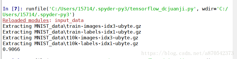
print (accuracy.eval(feed_dict={x: mnist.test.images, y_: mnist.test.labels}))

这个下来的是大概91%的正确率

三、多层卷积网络

#深度卷积神经网络
#第一部：加载MNIST数据
import input_data
mnist = input_data.read_data_sets('MNIST_data', one_hot=True)
#InteractiveSession类。
#通过它，你可以更加灵活地构建你的代码。它能让你在运行图的时候，插入一些计算图，这些计算图是由某些操作(operations)构成的。
#第二部分：变量的定义
import tensorflow as tf
sess = tf.InteractiveSession()
#占位符placeholder
#虽然placeholder的shape参数是可选的，但有了它，TensorFlow能够自动捕捉因数据维度不一致导致的错误。
x = tf.placeholder("float", shape=[None, 784])
y_ = tf.placeholder("float", shape=[None, 10])
#变量权重W和偏置b Variable
W = tf.Variable(tf.zeros([784,10]))
b = tf.Variable(tf.zeros([10]))
#变量需要通过seesion初始化后，才能在session中使用。
#这一初始化步骤为，为初始值指定具体值（本例当中是全为零），并将其分配给每个变量,可以一次性为所有变量完成此操作。
sess.run(tf.initialize_all_variables())

#构建一个多层卷积网络
#权重初始化
def weight_variable(shape):
initial = tf.truncated_normal(shape, stddev=0.1)
return tf.Variable(initial)

def bias_variable(shape):
initial = tf.constant(0.1, shape=shape)
return tf.Variable(initial)

#卷积和池化
def conv2d(x, W):
return tf.nn.conv2d(x, W, strides=[1, 1, 1, 1], padding='SAME')

def max_pool_2x2(x):
return tf.nn.max_pool(x, ksize=[1, 2, 2, 1],
strides=[1, 2, 2, 1], padding='SAME')
#第一层卷积
W_conv1 = weight_variable([5, 5, 1, 32])
b_conv1 = bias_variable([32])

x_image = tf.reshape(x, [-1,28,28,1])

h_conv1 = tf.nn.relu(conv2d(x_image, W_conv1) + b_conv1)
h_pool1 = max_pool_2x2(h_conv1)

#第二层卷积
W_conv2 = weight_variable([5, 5, 32, 64])
b_conv2 = bias_variable([64])

h_conv2 = tf.nn.relu(conv2d(h_pool1, W_conv2) + b_conv2)
h_pool2 = max_pool_2x2(h_conv2)
#密集连接层
W_fc1 = weight_variable([7 * 7 * 64, 1024])
b_fc1 = bias_variable([1024])

h_pool2_flat = tf.reshape(h_pool2, [-1, 7*7*64])
h_fc1 = tf.nn.relu(tf.matmul(h_pool2_flat, W_fc1) + b_fc1)
#Dropout
keep_prob = tf.placeholder("float")
h_fc1_drop = tf.nn.dropout(h_fc1, keep_prob)
#输出层
W_fc2 = weight_variable([1024, 10])
b_fc2 = bias_variable([10])

y_conv=tf.nn.softmax(tf.matmul(h_fc1_drop, W_fc2) + b_fc2)
#训练和评估模型
cross_entropy = -tf.reduce_sum(y_*tf.log(y_conv))
train_step = tf.train.AdamOptimizer(1e-4).minimize(cross_entropy)
correct_prediction = tf.equal(tf.argmax(y_conv,1), tf.argmax(y_,1))
accuracy = tf.reduce_mean(tf.cast(correct_prediction, "float"))
sess.run(tf.initialize_all_variables())
for i in range(20000):
batch = mnist.train.next_batch(50)
if i%100 == 0:
    train_accuracy = accuracy.eval(feed_dict={
        x:batch[0], y_: batch[1], keep_prob: 1.0})
    print( "step %d, training accuracy %g"%(i, train_accuracy))
train_step.run(feed_dict={x: batch[0], y_: batch[1], keep_prob: 0.5})

print ("test accuracy %g"%accuracy.eval(feed_dict={
x: mnist.test.images, y_: mnist.test.labels, keep_prob: 1.0}))

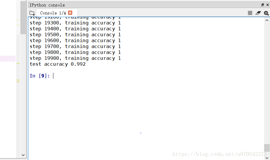
正确率为99.2%