Python实现直方图的绘制

Python实现直方图的绘制：

说明：代码运行环境：Win10+Python3+jupyter notebook

直方图简介：

直方图是一种常用的数量型数据的图形描述方法。它的一个最重要应用是提供了数据的分布形态的信息。

 

直方图主要的绘制方法：

方法1：通过pandas包中的调用Series对象或DataFrame对象的plot()、plot.hist()或hist()方法

方法2：通过matplotlib包中的Axes对象调用hist()方法创建直方图：

首先导出需要的各种包，并准备好数据：

%matplotlib notebook

import pandas as pd
import matplotlib.pyplot as plot
import numpy as np

tips = pd.read_csv('examples/tips.csv')
tips['tip_pct']=tips['tip']/(tips['total_bill']-tips['tip']) # 向tips 中添加'tip_pct'列

加入'tip_pct'列后的tips表的结构如下图所示：

开始绘制直方图：

方法1具体示例：

Series.plot.hist()示例：

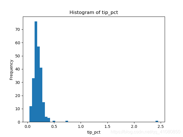
fig,axes = plt.subplots()
tips['tip_pct'].plot.hist(bins=50,ax=axes)
axes.set_title('Histogram of tip_pct')  #设置直方图的标题
axes.set_xlabel('tip_pct')              # 设置直方图横坐标轴的标签
plt.savefig('p1.png')  # 保存图片

上述代码绘制的图形为：

Series.plot.hist()的用法具体参考：

https://pandas.pydata.org/pandas-docs/stable/generated/pandas.Series.plot.hist.html

Series.plot(kind='hist')的用法与Series.plot.hist()类似，具体参考：

https://pandas.pydata.org/pandas-docs/stable/generated/pandas.Series.plot.html#pandas.Series.plot

DataFrame.plot.hist()示例：

fig,axes = plt.subplots(2,2)
tips.plot.hist(bins=50,subplots=True,ax=axes,legend=False)

axes[0,0].set_title('Histogram og total bill')
axes[0,0].set_xlabel('total_bill')
axes[0,1].set_title('Histogram of tip')
axes[0,1].set_xlabel('tip')
axes[1,0].set_title('Histogram of size')
axes[1,0].set_xlabel('size')
axes[1,1].set_title('Histogram of tip_pct')
axes[1,1].set_xlabel('tip_pct')

plt.subplots_adjust(wspace=0.5,hspace=0.5)  # 调整axes中各个子图之间的间距

plt.savefig('p2.png')      

上述代码绘制的图形为：

可以看到，上图中四个子图的横坐标范围是完全相同的，DataFrame.plot.hist不会根据各个子图中的数据自动调整横坐标轴上数值的范围。与DataFrame.plot.hist()方法相比，DataFrame.hist()会根据不同数据自动调整横坐标轴上的的数值范围，使用起来更加的方便。

DataFrame.plot.hist()的用法具体参考：

https://pandas.pydata.org/pandas-docs/stable/generated/pandas.DataFrame.plot.hist.html

DataFrame.plot(kind='hist')的用法与DataFrame.plot.hist()类似，具体参考：

ttps://pandas.pydata.org/pandas-docs/stable/generated/pandas.DataFrame.plot.html

DataFrame.hist()示例：

fig,axes = plt.subplots(2,2)
tips.hist(column='total_bill',ax=axes[0,0],bins=50)
axes[0,0].set_title('Histogram of total_bill')
axes[0,0].set_xlabel('total_bill')

tips.hist(column='tip',ax=axes[0,1],bins=50)
axes[0,1].set_title('Histogram of tip')
axes[0,1].set_xlabel('tip')

tips.hist(column='size',ax=axes[1,0],bins=50)
axes[1,0].set_title('Histogram of size')
axes[1,0].set_xlabel('size')

tips.hist(column='tip_pct',ax=axes[1,1],bins=50)
axes[1,1].set_title('Histogram of tip_pct')
axes[1,1].set_xlabel('tip_pct')

plt.subplots_adjust(wspace=0.42,hspace=0.42)
plt.savefig('p3.png')

上述代码绘制的图形为：

DataFrame.hist()的用法具体参考：

https://pandas.pydata.org/pandas-docs/stable/generated/pandas.DataFrame.hist.html#pandas.DataFrame.hist

Series.hist()示例：

fig,axes = plt.subplots(1,2)      # xrot表示x轴上数据标签的偏转角度
tips['tip_pct'].hist(by=tips['smoker'],ax=axes,bins=50,xrot=0.1)
axes[0].set_title('tip_pct of non-smoker ')
axes[0].set_xlabel('tip_pct')

axes[1].set_title('tip_pct of smoker ')
axes[1].set_xlabel('tip_pct')

plt.subplots_adjust(wspace=0.4,hspace=0.4)
plt.savefig('p4.png')

 上述代码绘制的图形为：

Series.hist()的用法具体参考：

https://pandas.pydata.org/pandas-docs/stable/generated/pandas.Series.hist.html#pandas.Series.hist

 

方法2具体示例：

Axes.hist()的用法具体参考：

https://matplotlib.org/api/_as_gen/matplotlib.axes.Axes.hist.html#matplotlib.axes.Axes.hist

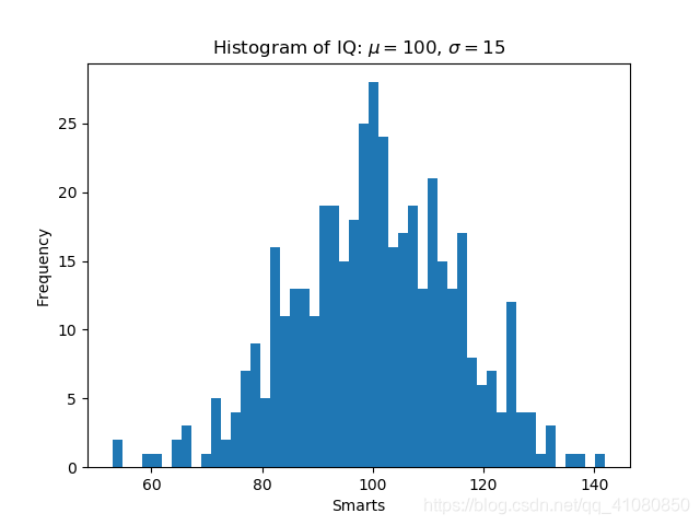
频数分布直方图示例：

import numpy as np
import matplotlib.pyplot as plt

np.random.seed(19680801)  # 让每次生成的随机数相同

# 示例数据
mu = 100  # 数据均值
sigma = 15  # 数据标准差
x = mu + sigma * np.random.randn(437)

num_bins = 50

fig, ax = plt.subplots()   # 等价于fig, ax = plt.subplots(1,1)

# 数据的频数分布直方图
n, bins, patches = ax.hist(x, num_bins,density=False)
# n是一个数组或者由数组组成的列表，表示落在每个分组中的数据的频数
# bins是一个数组，表示每个分组的边界，一共有50个组，所以bins的长度就是51
# patches是一个列表或者嵌套列表，长度是50,,列表里的元素可以理解成直方图中的小长方条

ax.set_xlabel('Smarts')
ax.set_ylabel('Frequency')
ax.set_title(r'Histogram of IQ: $\mu=100$, $\sigma=15$')
plt.savefig('p5.png')

上述代码绘制的图形为：

频率分布直方图示例：

np.random.seed(19680801)  # 让每次生成的随机数相同

# 示例数据
mu = 100  # 数据均值
sigma = 15  # 数据标准差
x = mu + sigma * np.random.randn(437)

num_bins = 50

fig, ax = plt.subplots()   # 等价于fig, ax = plt.subplots(1,1)

# 数据的频率分布直方图

n, bins, patches = ax.hist(x, num_bins,density=True)
# n是一个数组或者由数组组成的列表，表示落在每个分组中的数据的频数
# bins是一个数组，表示每个分组的边界，一共有50个组，所以bins的长度就是51
# patches是一个列表或者嵌套列表，长度是50,,列表里的元素可以理解成直方图中的小长方条

ax.set_xlabel('Smarts')
ax.set_ylabel('Probability density') # 频率分布直方图的纵轴表示的是频率/组距
ax.set_title(r'Histogram of IQ: $\mu=100$, $\sigma=15$')

plt.savefig('p6.png')

上述代码绘制的图形为：

如何给直方图中的长条添加数据标记？

np.random.seed(19680801)  # 让每次生成的随机数相同

# 示例数据
mu = 100  # 数据均值
sigma = 15  # 数据标准差
x = mu + sigma * np.random.randn(437)
num_bins = 5  # 为了便于给直方图中的长条添加数据标签，将数据分成五组
fig, ax = plt.subplots()   # 等价于fig, ax = plt.subplots(1,1)

# 数据的频率分布直方图(带数据标签)
n, bins, patches = ax.hist(x, num_bins,density=True)
# n是一个数组或者由数组组成的列表，表示落在每个分组中的数据的频数
# bins是一个数组，表示每个分组的边界，一共有50个组，所以bins的长度就是51
# patches是一个列表或者嵌套列表，长度是50,,列表里的元素可以理解成直方图中的小长方条

# 写一个给直方图中的长条添加数据标签的函数
def data_marker(patches):
    for patch in patches:
        height = patch.get_height()
        if height != 0:
            ax.text(patch.get_x() + patch.get_width()/4, height + 0.0002,'{:.5f}'.format(height))             

data_marker(patches)   # 调用data_marker函数

ax.set_xlabel('Smarts')
ax.set_ylabel('Probability density') # 频率分布直方图的纵轴表示的是频率/组距
ax.set_title(r'Histogram of IQ: $\mu=100$, $\sigma=15$')
plt.savefig('p7.png')       #  保存生成的图片

上述代码绘制的图形为：

参考资料：

《Python for Data Analysis》第二版

https://blog.csdn.net/a821235837/article/details/52839050

https://wenku.baidu.com/view/036fea38aef8941ea66e052f.html

https://blog.csdn.net/yywan1314520/article/details/50818471

matplotlib、pandas官方文档

PS：本文为博主原创文章，转载请注明出处。