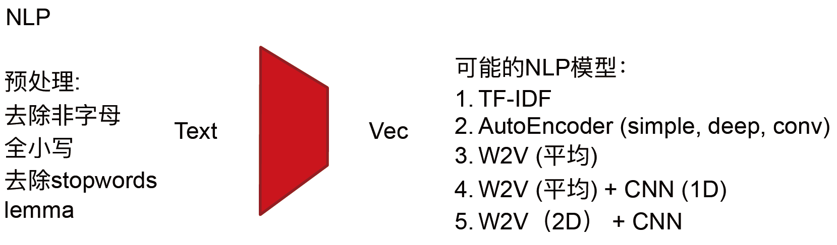
Auto-Encoder

如果原始图片输入后经过神经网络压缩成中间状态(编码过程Encoder),再由中间状态解码出的图片与原始输入差别很小(D解码过程ecoder),那么这个中间状态的东西,就可以用来表示原始的输入。
原先打算用AE来做神经网络中的W,但是发现效果不好,然后神经网络使用batch 的方法来平滑损失函数曲线,然后使用神经网络的“跳层”方法优化神经网络。
所以AE用处最多的就是降维。
有一个问题,农场主假设,如果一群鸡每天10点喂食,那么鸡中比较聪明的鸡就会认为每天10点钟有食物是一种自然规律,这个鸡认为的这种自然规律在机器学习中叫做局部最优解,也就是过拟合。
同理,人类在认知世界的过程中,无法开启上帝之眼,无法跳出三维而完全的认识三维世界。

AE实现过程:
from keras.layers import Input, Dense
from keras.models import Model
from sklearn.cluster import KMeans


class ASCIIAutoencoder():
    """基于字符的Autoencoder."""

    def __init__(self, sen_len = 512, encoding_dim = 32, epoch = 50, val_ratio = 0.3):
        """
        Init.
        :param sen_len: 把sentences pad成相同的⻓长度
        :param encoding_dim: 压缩后的维度dim
        :param epoch: 要跑多少epoch
        :param kmeanmodel: 简单的KNN clustering模型
        """
        self.sen_len = sen_len
        self.encoding_dim = encoding_dim
        self.autoencoder = None
        self.encoder = None
        self.kmeanmodel = KMeans(n_clusters = 2)
        self.epoch = epoch

    def fit(self, x):
        """
        模型构建。
        :param x: input text
        """
        # 把所有的trainset都搞成同⼀一个size,并把每⼀一个字符都换成ascii码
        x_train = self.preprocess(x, length = self.sen_len)
        # 然后给input预留留好位置
        input_text = Input(shape = (self.sen_len,))
        # "encoded" 每⼀一经过⼀一层,都被刷新成⼩小⼀一点的“压缩后表达式”
        encoded = Dense(1024, activation = 'tanh')(input_text)
        encoded = Dense(512, activation = 'tanh')(encoded)
        encoded = Dense(128, activation = 'tanh')(encoded)
        encoded = Dense(self.encoding_dim, activation = 'tanh')(encoded)
        # "decoded" 就是把刚刚压缩完的东⻄西,给反过来还原成input_text
        decoded = Dense(128, activation = 'tanh')(encoded)
        decoded = Dense(512, activation = 'tanh')(decoded)
        decoded = Dense(1024, activation = 'tanh')(decoded)
        decoded = Dense(self.sen_len, activation = 'sigmoid')(decoded)
        # 整个从⼤大到⼩小再到⼤大的model,叫 autoencoder
        self.autoencoder = Model(input = input_text, output = decoded)
        # 那么 只从⼤大到⼩小(也就是⼀一半的model)就叫 encoder
        self.encoder = Model(input = input_text, output = encoded)
        # 同理理,我们接下来搞⼀一个decoder出来,也就是从⼩小到⼤大的model
        # 来,首先encoded的input size给预留留好
        encoded_input = Input(shape = (1024,))
        # autoencoder的最后⼀一层,就应该是decoder的第⼀一层
        decoder_layer = self.autoencoder.layers[-1]
        # 然后我们从头到尾连起来,就是⼀一个decoder了了!
        decoder = Model(input = encoded_input, output = decoder_layer(encoded_input))
        # compile
        self.autoencoder.compile(optimizer = 'adam', loss = 'mse')
        # 跑起来
        self.autoencoder.fit(x_train, x_train,
                             nb_epoch = self.epoch,
                             batch_size = 1000,
                             shuffle = True,
                             )
        # 这⼀一部分是⾃自⼰己拿⾃自⼰己train⼀一下KNN,⼀一件简单的基于距离的分类器器
        x_train = self.encoder.predict(x_train)
        self.kmeanmodel.fit(x_train)

    def predict(self, x):
        """
        做预测。
        :param x: input text
        :return: predictions
        """
        # 同理理,第⼀一步 把来的 都给搞成ASCII化,并且⻓长度相同
        x_test = self.preprocess(x, length = self.sen_len)
        # 然后⽤用encoder把test集给压缩
        x_test = self.encoder.predict(x_test)
        # KNN给分类出来
        preds = self.kmeanmodel.predict(x_test)
        return preds

    def preprocess(self, s_list, length = 256):
        ...
CNN4Text

如何迁移到文字处理理?
1. 把文字表示成图片
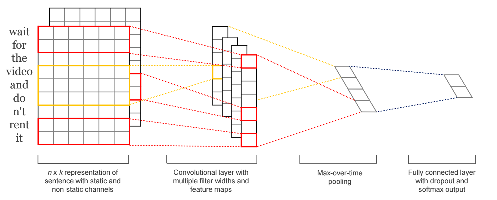
也可以把句子做成一维的:

CNN假设:
RNN假设:
边界处理理:
Narrow vs Wide
Stride size:
步伐大小
# 有两种⽅方法可以做CNN for text
# 每种⽅方法⾥里里⾯面,也有各种不不同的玩法思路路
# 效果其实基本都差不不多,
# 我这⾥里里讲2种最普遍的:
# 1. ⼀一维的vector [...] + ⼀一维的filter [...]
# 这种⽅方法有⼀一定的信息损失(因为你average了了向量量),但是速度快,效果也没太差。
# 2. 通过w2v或其他⽅方法,做成⼆二维matrix,当做图⽚片来做。
# 这是⽐比较“讲道理理”的解决⽅方案,但是就是慢。。。放AWS上太烧钱了了。。。
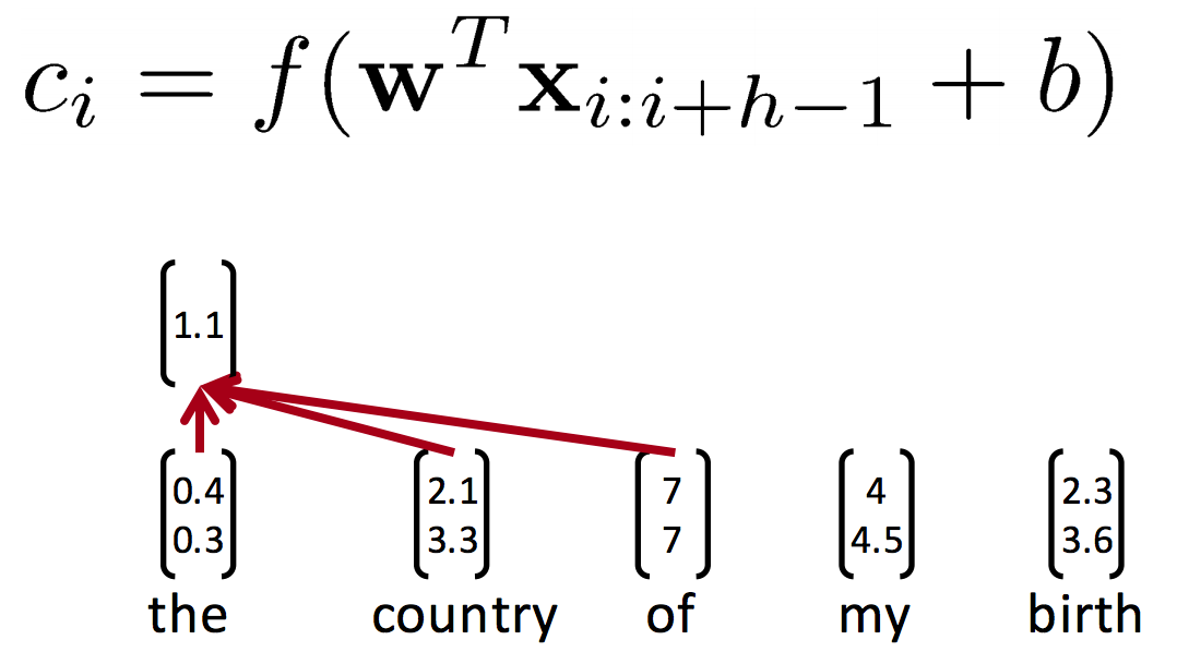
# 1. 1D CNN for Text
# ⼀一个IMDB电影评论的例例⼦子
import numpy as np
np.random.seed(1337) # for reproducibility
from keras.preprocessing import sequence
from keras.models import Sequential
from keras.layers import Dense, Dropout, Activation, Flatten
from keras.layers import Embedding
from keras.layers import Convolution1D, MaxPooling1D
from keras.datasets import imdb
# set parameters:
max_features = 5000
maxlen = 400
batch_size = 32
embedding_dims = 50
nb_filter = 250
filter_length = 3
hidden_dims = 250
nb_epoch = 2
# ⾃自带的数据集,load IMDB data
(X_train, y_train), (X_test, y_test) = imdb.load_data(nb_words = max_features)
# 这个数据集是已经搞好了了的BoW,⻓长这样:
# [123, 2, 0, 45, 32, 1212, 344, 4, ... ]
# 简单的把他们搞成相同⻓长度,不不够的补0,太多的砍掉
X_train = sequence.pad_sequences(X_train, maxlen = maxlen)
X_test = sequence.pad_sequences(X_test, maxlen = maxlen)
# 这⾥里里我们可以换成word2vec的vector,他们就是天然的相同⻓长度了了
# 留留个作业,⼤大家可以试试
# 初始化我们的sequential model (指的是线性排列列的layer)
model = Sequential()
# 亮点来了了,这⾥里里你需要⼀一个Embedding Layer来把你的input word indexes
# 变成tensor vectors: ⽐比如 如果dim是3, 那么:
# [[2],[123], ...] --> [[0.1, 0.4, 0.21], [0.2, 0.4, 0.13], ... ]
# 其实很像word2vec的结果,只不不过这个Embedding没有什什么太⼤大意义,只是向量量化了了input的int
model.add(Embedding(max_features,
embedding_dims,
input_length = maxlen,
dropout = 0.2))
# 这⼀一步对于直接⽤用BoW(⽐比如这个IMDB的数据集)很⽅方便便,但是对我们⾃自⼰己的word vector,
# 就不不友好了了,可以选择跳过它
# 现在可以添加⼀一个Conv layer了了
model.add(Convolution1D(nb_filter = nb_filter, filter_length = filter_length, border_mode = 'valid',
activation = 'relu', subsample_length = 1))
# 后⾯面跟⼀一个MaxPooling
model.add(MaxPooling1D(pool_length = model.output_shape[1]))
# Pool出来的结果 就是类似于⼀一堆的⼩小vec
# 把他们粗暴暴的flatten⼀一下(就是横着 连成⼀一起)
model.add(Flatten())
# 接下来就是简单的MLP了了
# 在Keras⾥里里,普通的layer⽤用Dense表示
model.add(Dense(hidden_dims))
model.add(Dropout(0.2))
model.add(Activation('relu'))
# 最终层
model.add(Dense(1))
model.add(Activation('sigmoid'))
# 如果⾯面对的是时间序列列的话,
# 这⾥里里也是可以把layers都换成LSTM
# compile
model.compile(loss = 'binary_crossentropy', optimizer = 'adam', metrics = ['accuracy'])
# 跑起来
model.fit(X_train, y_train,
batch_size = batch_size,
nb_epoch = nb_epoch,
validation_data = (X_test, y_test))
# 这⾥里里有个fault啊,不不可以拿testset做validation的
# 这只是简单的做个示例例,为了了跑起来⽅方便便
# 2. 2D CNN
# 我们的input 应该是⼀一个list of M*N matrixs
# 但是注意⼀一下,我们需要稍微reshape⼀一下,把每个matrix⽤用⼀一个⼀一维的[]包起来
# 这就等于 我们把input变成 list of lists, 每个list包含⼀一个M*N Matrix
x_train = X_train.reshape(X_train.shape[0], 1,
X_train.shape[1], X_train.shape[2])
# cast⼀一下type,以防Numpy冲突
x_train = x_train.astype('float32')
# 接着,还是⼀一样:
model = Sequential()
# n_filter, ⼀一共⼏几个filter
# n_conv,每个filter的size
model.add(Convolution2D(n_filter, n_conv, n_conv,
border_mode = border_mode,
input_shape = (1, x_axis,
y_axis)))
model.add(Activation('relu'))
model.add(Convolution2D(n_filter, n_conv, n_conv))
model.add(Activation('relu'))
model.add(MaxPooling2D(pool_size = (n_pool, n_pool)))
model.add(Dropout(0.25))
model.add(Flatten())
案例
从每日新闻中预测金融市场变化
数据获取
/r/worldnews

DJIA(道琼斯指数)

RedditNews(经济新闻)

Combine
Date, Text, Label
W2V模型的Pretrain:
1.GoogleNews.bin (https://code.google.com/archive/p/word2vec/)
2.RedditComments (https://www.reddit.com/r/datasets/comments/3mg812/full_reddit_submission_corpus_now_available_2006/)
3. 用我提供的dataset里的新闻文本直接当场train
4. 我预先训练好的 reddit w2v model
ML
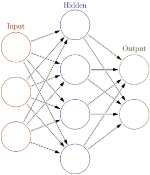
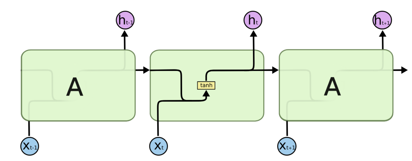
普通神经网络:
RNN:
RNN的目的是让有sequential关系的信息得到考虑。
什么是sequential关系?
就是信息在时间上的前后关系。
相比于普通神经网络:
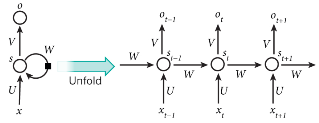
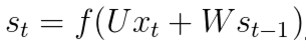
每个时间点中的S计算
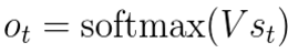
这个神经元最终的输出,
基于最后一个S
简单来说,对于t=5来说,其实就相当于把一个神经元拉伸成五个
换句句话说,S就是我们所说的记忆(因为把t从1-5的信息都记录下来了)
由前文可见,RNN可以带上记忆。
假设,一个『生成下一个单词』的例子:
『这顿饭真好』——>『吃』
很明显,我们只要前5个字就能猜到下一个字是啥了了
However,
如果我问你,『穿山甲说了什么?』
你能回答嘛?
(credit to 暴走漫画)
LSTM
RNN
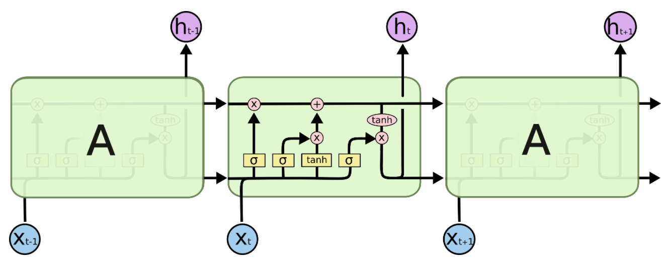
LSTM
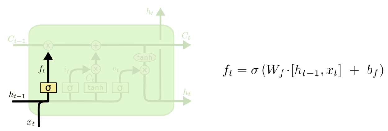
LSTM中最重要的就是这个Cell State,它一路向下,贯穿这个时间线,代表了记忆的纽带。它会被XOR和AND运算符搞一搞,来更更新记忆
而控制信息的增加和减少的,就是靠这些阀门:Gate
阀门嘛,就是输出一个1于0之间的值:
1 代表,把这一趟的信息都记着
0 代表,这一趟的信息可以忘记了
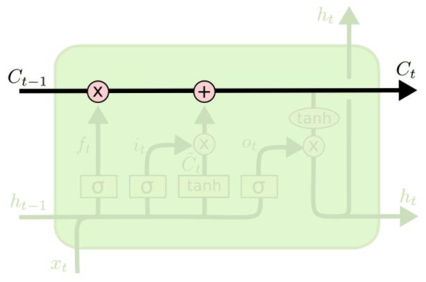
下面我们来模拟一遍信息在LSTM里跑跑~
第一步:忘记门
来决定我们该忘记什么信息
它把上一次的状态ht-1和这一次的输入xt相比较
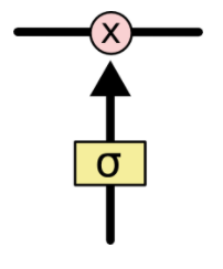
通过gate输出一个0到1的值(就像是个activation function一样),
1 代表:给我记着!
0 代表:快快忘记!
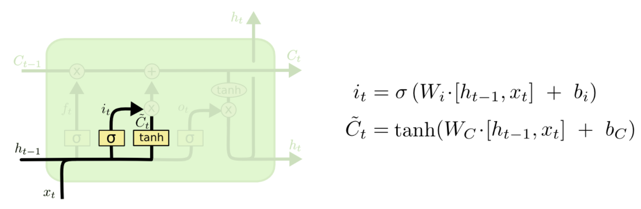
第二步:记忆门
哪些该记住
这个门比较复杂,分两步:
第一步,用sigmoid决定什什么信息需要被我们更新(忘记旧的)
第二部,用Tanh造一个新的Cell State(更更新后的cell state)
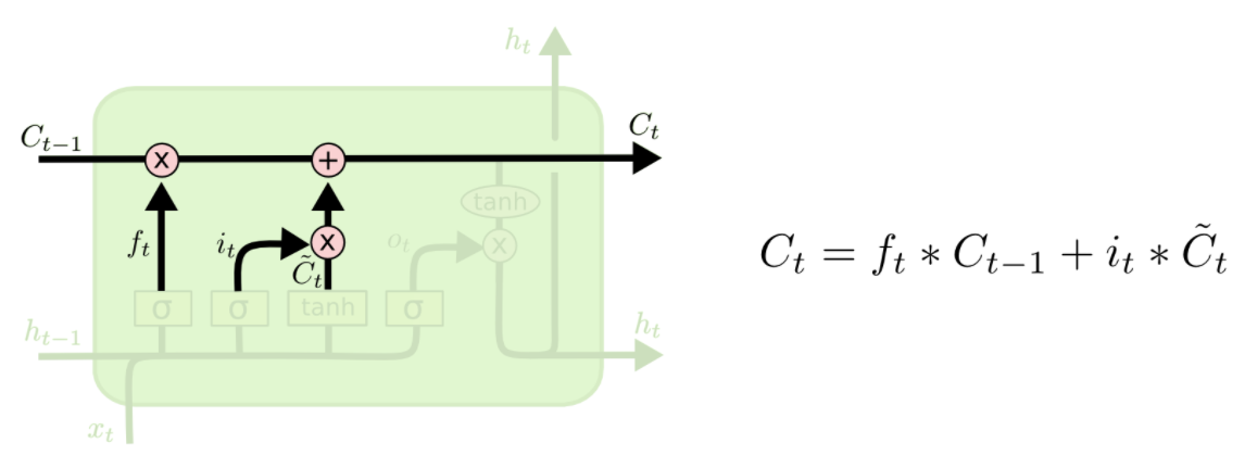
第三步:更新门
把老cell state更新为新cell state
用XOR和AND这样的门来更新我们的cell state:
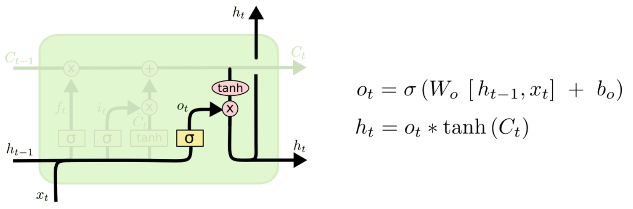
第四步:输出门
由记忆来决定输出什什么值
我们的Cell State已经被更更新,
于是我们通过这个记忆纽带,来决定我们的输出:
(这里的Ot类似于我们刚刚RNN里里直接一步跑出来的output)
案例
题目原型:What’s Next?
可以用在不不同的维度上:
维度1:下一个字母是什么?
维度2:下一个单词是什么?
维度3:下一个句子是什么?
维度N:下一个图片/音符/….是什么?
用RNN做文本生成
举个小小的例子,来看看LSTM是怎么玩的
我们这里用温斯顿丘吉尔的人物传记作为我们的学习语料。
第一步,一样,先导入各种库
import numpy
from keras.models import Sequential
from keras.layers import Dense
from keras.layers import Dropout
from keras.layers import LSTM
from keras.callbacks import ModelCheckpoint
from keras.utils import np_utils
Using Theano backend.
Using gpu device 0: Tesla K80 (CNMeM is disabled, cuDNN 5105)
/usr/local/lib/python3.5/dist-packages/theano/sandbox/cuda/__init__.py:600: UserWarning: Your cuDNN version is more recent than the one Theano officially supports. If you see any problems, try updating Theano or downgrading cuDNN to version 5.
  warnings.warn(warn)
接下来,我们把文本读入
raw_text = open('../input/Winston_Churchil.txt').read()
raw_text = raw_text.lower()
既然我们是以每个字母为层级,字母总共才26个,所以我们可以很方便的用One-Hot来编码出所有的字母(当然,可能还有些标点符号和其他noise)
chars = sorted(list(set(raw_text)))
char_to_int = dict((c, i) for i, c in enumerate(chars))
int_to_char = dict((i, c) for i, c in enumerate(chars))
我们看到,全部的chars:
chars
一共有:
len(chars)
61
同时,我们的原文本一共有:
len(raw_text)
我们这里简单的文本预测就是,给了前置的字母以后,下一个字母是谁?
比如,Winsto, 给出 n Britai 给出 n
构造训练测试集
我们需要把我们的raw text变成可以用来训练的x,y:
x 是前置字母们 y 是后一个字母
seq_length = 100
x = []
y = []
for i in range(0, len(raw_text) - seq_length):
    given = raw_text[i:i + seq_length]
    predict = raw_text[i + seq_length]
    x.append([char_to_int[char] for char in given])
    y.append(char_to_int[predict])
我们可以看看我们做好的数据集的长相:
print(x[:3])
print(y[:3])
[[60, 45, 47, 44, 39, 34, 32, 49, 1, 36, 50, 49, 34, 43, 31, 34, 47, 36, 57, 48, 1, 47, 34, 30, 41, 1, 48, 44, 41, 33, 38, 34, 47, 48, 1, 44, 35, 1, 35, 44, 47, 49, 50, 43, 34, 9, 1, 31, 54, 1, 47, 38, 32, 37, 30, 47, 33, 1, 37, 30, 47, 33, 38, 43, 36, 1, 33, 30, 51, 38, 48, 0, 0, 49, 37, 38, 48, 1, 34, 31, 44, 44, 40, 1, 38, 48, 1, 35, 44, 47, 1, 49, 37, 34, 1, 50, 48, 34, 1, 44], [45, 47, 44, 39, 34, 32, 49, 1, 36, 50, 49, 34, 43, 31, 34, 47, 36, 57, 48, 1, 47, 34, 30, 41, 1, 48, 44, 41, 33, 38, 34, 47, 48, 1, 44, 35, 1, 35, 44, 47, 49, 50, 43, 34, 9, 1, 31, 54, 1, 47, 38, 32, 37, 30, 47, 33, 1, 37, 30, 47, 33, 38, 43, 36, 1, 33, 30, 51, 38, 48, 0, 0, 49, 37, 38, 48, 1, 34, 31, 44, 44, 40, 1, 38, 48, 1, 35, 44, 47, 1, 49, 37, 34, 1, 50, 48, 34, 1, 44, 35], [47, 44, 39, 34, 32, 49, 1, 36, 50, 49, 34, 43, 31, 34, 47, 36, 57, 48, 1, 47, 34, 30, 41, 1, 48, 44, 41, 33, 38, 34, 47, 48, 1, 44, 35, 1, 35, 44, 47, 49, 50, 43, 34, 9, 1, 31, 54, 1, 47, 38, 32, 37, 30, 47, 33, 1, 37, 30, 47, 33, 38, 43, 36, 1, 33, 30, 51, 38, 48, 0, 0, 49, 37, 38, 48, 1, 34, 31, 44, 44, 40, 1, 38, 48, 1, 35, 44, 47, 1, 49, 37, 34, 1, 50, 48, 34, 1, 44, 35, 1]]
[35, 1, 30]
此刻,楼上这些表达方式,类似就是一个词袋,或者说 index。
接下来我们做两件事:
-
我们已经有了一个input的数字表达(index),我们要把它变成LSTM需要的数组格式: [样本数,时间步伐,特征]
-
第二,对于output,我们在Word2Vec里学过,用one-hot做output的预测可以给我们更好的效果,相对于直接预测一个准确的y数值的话。
n_patterns = len(x)
n_vocab = len(chars)

# 把x变成LSTM需要的样子
x = numpy.reshape(x, (n_patterns, seq_length, 1))
# 简单normal到0-1之间
x = x / float(n_vocab)
# output变成one-hot
y = np_utils.to_categorical(y)

print(x[11])
print(y[11])
[[ 0.80327869]
 [ 0.55737705]
 [ 0.70491803]
 [ 0.50819672]
 [ 0.55737705]
 [ 0.7704918 ]
 [ 0.59016393]
 [ 0.93442623]
 [ 0.78688525]
 [ 0.01639344]
 [ 0.7704918 ]
 [ 0.55737705]
 [ 0.49180328]
 [ 0.67213115]
 [ 0.01639344]
 [ 0.78688525]
 [ 0.72131148]
 [ 0.67213115]
 [ 0.54098361]
 [ 0.62295082]
 [ 0.55737705]
 [ 0.7704918 ]
 [ 0.78688525]
 [ 0.01639344]
 [ 0.72131148]
 [ 0.57377049]
 [ 0.01639344]
 [ 0.57377049]
 [ 0.72131148]
 [ 0.7704918 ]
 [ 0.80327869]
 [ 0.81967213]
 [ 0.70491803]
 [ 0.55737705]
 [ 0.14754098]
 [ 0.01639344]
 [ 0.50819672]
 [ 0.8852459 ]
 [ 0.01639344]
 [ 0.7704918 ]
 [ 0.62295082]
 [ 0.52459016]
 [ 0.60655738]
 [ 0.49180328]
 [ 0.7704918 ]
 [ 0.54098361]
 [ 0.01639344]
 [ 0.60655738]
 [ 0.49180328]
 [ 0.7704918 ]
 [ 0.54098361]
 [ 0.62295082]
 [ 0.70491803]
 [ 0.59016393]
 [ 0.01639344]
 [ 0.54098361]
 [ 0.49180328]
 [ 0.83606557]
 [ 0.62295082]
 [ 0.78688525]
 [ 0.        ]
 [ 0.        ]
 [ 0.80327869]
 [ 0.60655738]
 [ 0.62295082]
 [ 0.78688525]
 [ 0.01639344]
 [ 0.55737705]
 [ 0.50819672]
 [ 0.72131148]
 [ 0.72131148]
 [ 0.6557377 ]
 [ 0.01639344]
 [ 0.62295082]
 [ 0.78688525]
 [ 0.01639344]
 [ 0.57377049]
 [ 0.72131148]
 [ 0.7704918 ]
 [ 0.01639344]
 [ 0.80327869]
 [ 0.60655738]
 [ 0.55737705]
 [ 0.01639344]
 [ 0.81967213]
 [ 0.78688525]
 [ 0.55737705]
 [ 0.01639344]
 [ 0.72131148]
 [ 0.57377049]
 [ 0.01639344]
 [ 0.49180328]
 [ 0.70491803]
 [ 0.8852459 ]
 [ 0.72131148]
 [ 0.70491803]
 [ 0.55737705]
 [ 0.01639344]
 [ 0.49180328]
 [ 0.70491803]]
[ 0.  0.  0.  0.  0.  0.  0.  0.  0.  0.  0.  0.  0.  0.  0.  0.  0.  0.
  0.  0.  0.  0.  0.  0.  0.  0.  0.  0.  0.  0.  0.  0.  0.  0.  0.  0.
  0.  0.  0.  0.  0.  0.  0.  0.  0.  0.  0.  0.  0.  0.  0.  0.  0.  0.
  1.  0.  0.  0.  0.  0.]
模型建造
LSTM模型构建
model = Sequential()
model.add(LSTM(256, input_shape=(x.shape[1], x.shape[2])))
model.add(Dropout(0.2))
model.add(Dense(y.shape[1], activation='softmax'))
model.compile(loss='categorical_crossentropy', optimizer='adam')
跑模型
model.fit(x, y, nb_epoch=50, batch_size=4096)
我们来写个程序,看看我们训练出来的LSTM的效果:
def predict_next(input_array):
    x = numpy.reshape(input_array, (1, seq_length, 1))
    x = x / float(n_vocab)
    y = model.predict(x)
    return y

def string_to_index(raw_input):
    res = []
    for c in raw_input[(len(raw_input)-seq_length):]:
        res.append(char_to_int[c])
    return res

def y_to_char(y):
    largest_index = y.argmax()
    c = int_to_char[largest_index]
    return c
好,写成一个大程序:
def generate_article(init, rounds=200):
    in_string = init.lower()
    for i in range(rounds):
        n = y_to_char(predict_next(string_to_index(in_string)))
        in_string += n
    return in_string
init = 'His object in coming to New York was to engage officers for that service. He came at an opportune moment'
article = generate_article(init)
print(article)
his object in coming to new york was to engage officers for that service. he came at an opportune moment th the toote of the carie and the soote of the carie and the soote of the carie and the soote of the carie and the soote of the carie and the soote of the carie and the soote of the carie and the soo
用RNN做文本生成
举个小小的例子,来看看LSTM是怎么玩的
我们这里不再用char级别,我们用word级别来做。
第一步,一样,先导入各种库
import os
import numpy as np
import nltk
from keras.models import Sequential
from keras.layers import Dense
from keras.layers import Dropout
from keras.layers import LSTM
from keras.callbacks import ModelCheckpoint
from keras.utils import np_utils
from gensim.models.word2vec import Word2Vec
接下来,我们把文本读入
raw_text = ''
for file in os.listdir("../input/"):
    if file.endswith(".txt"):
        raw_text += open("../input/"+file, errors='ignore').read() + '\n\n'
# raw_text = open('../input/Winston_Churchil.txt').read()
raw_text = raw_text.lower()
sentensor = nltk.data.load('tokenizers/punkt/english.pickle')
sents = sentensor.tokenize(raw_text)
corpus = []
for sen in sents:
    corpus.append(nltk.word_tokenize(sen))

print(len(corpus))
print(corpus[:3])
91007
[['\ufeffthe', 'project', 'gutenberg', 'ebook', 'of', 'great', 'expectations', ',', 'by', 'charles', 'dickens', 'this', 'ebook', 'is', 'for', 'the', 'use', 'of', 'anyone', 'anywhere', 'at', 'no', 'cost', 'and', 'with', 'almost', 'no', 'restrictions', 'whatsoever', '.'], ['you', 'may', 'copy', 'it', ',', 'give', 'it', 'away', 'or', 're-use', 'it', 'under', 'the', 'terms', 'of', 'the', 'project', 'gutenberg', 'license', 'included', 'with', 'this', 'ebook', 'or', 'online', 'at', 'www.gutenberg.org', 'title', ':', 'great', 'expectations', 'author', ':', 'charles', 'dickens', 'posting', 'date', ':', 'august', '20', ',', '2008', '[', 'ebook', '#', '1400', ']', 'release', 'date', ':', 'july', ',', '1998', 'last', 'updated', ':', 'september', '25', ',', '2016', 'language', ':', 'english', 'character', 'set', 'encoding', ':', 'utf-8', '***', 'start', 'of', 'this', 'project', 'gutenberg', 'ebook', 'great', 'expectations', '***', 'produced', 'by', 'an', 'anonymous', 'volunteer', 'great', 'expectations', '[', '1867', 'edition', ']', 'by', 'charles', 'dickens', '[', 'project', 'gutenberg', 'editor’s', 'note', ':', 'there', 'is', 'also', 'another', 'version', 'of', 'this', 'work', 'etext98/grexp10.txt', 'scanned', 'from', 'a', 'different', 'edition', ']', 'chapter', 'i', 'my', 'father’s', 'family', 'name', 'being', 'pirrip', ',', 'and', 'my', 'christian', 'name', 'philip', ',', 'my', 'infant', 'tongue', 'could', 'make', 'of', 'both', 'names', 'nothing', 'longer', 'or', 'more', 'explicit', 'than', 'pip', '.'], ['so', ',', 'i', 'called', 'myself', 'pip', ',', 'and', 'came', 'to', 'be', 'called', 'pip', '.']]
好,w2v乱炖:
w2v_model = Word2Vec(corpus, size=128, window=5, min_count=5, workers=4)
可以了
w2v_model['office']
array([-0.01398709,  0.15975526,  0.03589381, -0.4449192 ,  0.365403  ,
        0.13376504,  0.78731823,  0.01640314, -0.29723561, -0.21117583,
        0.13451998, -0.65348488,  0.06038611, -0.02000343,  0.05698346,
        0.68013376,  0.19010596,  0.56921762,  0.66904438, -0.08069923,
       -0.30662233,  0.26082459, -0.74816126, -0.41383636, -0.56303871,
       -0.10834043, -0.10635001, -0.7193433 ,  0.29722607, -0.83104628,
        1.11914253, -0.34119046, -0.39490014, -0.34709939, -0.00583572,
        0.17824887,  0.43295503,  0.11827419, -0.28707108, -0.02838829,
        0.02565269,  0.10328653, -0.19100265, -0.24102989,  0.23023468,
        0.51493132,  0.34759828,  0.05510307,  0.20583512, -0.17160387,
       -0.10351282,  0.19884749, -0.03935663, -0.04055062,  0.38888735,
       -0.02003323, -0.16577065, -0.15858875,  0.45083243, -0.09268586,
       -0.91098118,  0.16775337,  0.3432925 ,  0.2103184 , -0.42439541,
        0.26097715, -0.10714807,  0.2415273 ,  0.2352251 , -0.21662289,
       -0.13343927,  0.11787982, -0.31010333,  0.21146733, -0.11726214,
       -0.65574747,  0.04007725, -0.12032496, -0.03468512,  0.11063002,
        0.33530036, -0.64098376,  0.34013858, -0.08341357, -0.54826909,
        0.0723564 , -0.05169795, -0.19633259,  0.08620321,  0.05993884,
       -0.14693044, -0.40531522, -0.07695422,  0.2279872 , -0.12342903,
       -0.1919964 , -0.09589464,  0.4433476 ,  0.38304719,  1.0319351 ,
        0.82628119,  0.3677327 ,  0.07600326,  0.08538571, -0.44261214,
       -0.10997667, -0.03823839,  0.40593523,  0.32665277, -0.67680383,
        0.32504487,  0.4009226 ,  0.23463745, -0.21442334,  0.42727917,
        0.19593567, -0.10731711, -0.01080817, -0.14738144,  0.15710345,
       -0.01099576,  0.35833639,  0.16394758, -0.10431164, -0.28202233,
        0.24488974,  0.69327635, -0.29230621], dtype=float32)
接下来,其实我们还是以之前的方式来处理我们的training data,把源数据变成一个长长的x,好让LSTM学会predict下一个单词:
raw_input = [item for sublist in corpus for item in sublist]
len(raw_input)
2115170
raw_input[12]
'ebook'
text_stream = []
vocab = w2v_model.vocab
for word in raw_input:
    if word in vocab:
        text_stream.append(word)
len(text_stream)
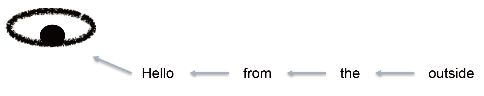
我们这里的文本预测就是,给了前面的单词以后,下一个单词是谁?
比如,hello from the other, 给出 side
构造训练测试集
我们需要把我们的raw text变成可以用来训练的x,y:
x 是前置字母们 y 是后一个字母
seq_length = 10
x = []
y = []
for i in range(0, len(text_stream) - seq_length):

    given = text_stream[i:i + seq_length]
    predict = text_stream[i + seq_length]
    x.append(np.array([w2v_model[word] for word in given]))
    y.append(w2v_model[predict])
我们可以看看我们做好的数据集的长相:
print(x[10])
print(y[10])
[[-0.02218935  0.04861801 -0.03001036 ...,  0.07096259  0.16345282
  -0.18007144]
 [ 0.1663752   0.67981642  0.36581406 ...,  1.03355932  0.94110376
  -1.02763569]
 [-0.12611888  0.75773817  0.00454156 ...,  0.80544478  2.77890372
  -1.00110698]
 ...,
 [ 0.34167829 -0.28152692 -0.12020591 ...,  0.19967555  1.65415502
  -1.97690392]
 [-0.66742641  0.82389861 -1.22558379 ...,  0.12269551  0.30856156
   0.29964617]
 [-0.17075984  0.0066567  -0.3894183  ...,  0.23729582  0.41993639
  -0.12582727]]
[ 0.18125793 -1.72401989 -0.13503326 -0.42429626  1.40763748 -2.16775346
  2.26685596 -2.03301549  0.42729807 -0.84830129  0.56945151  0.87243706
  3.01571465 -0.38155749 -0.99618471  1.1960727   1.93537641  0.81187075
 -0.83017075 -3.18952608  0.48388934 -0.03766865 -1.68608069 -1.84907544
 -0.95259917  0.49039507 -0.40943271  0.12804921  1.35876858  0.72395176
  1.43591952 -0.41952157  0.38778016 -0.75301784 -2.5016799  -0.85931653
 -1.39363682  0.42932403  1.77297652  0.41443667 -1.30974782 -0.08950856
 -0.15183811 -1.59824061 -1.58920395  1.03765178  2.07559252  2.79692245
  1.11855054 -0.25542653 -1.04980111 -0.86929852 -1.26279402 -1.14124119
 -1.04608357  1.97869778 -2.23650813 -2.18115139 -0.26534671  0.39432198
 -0.06398458 -1.02308178  1.43372631 -0.02581184 -0.96472031 -3.08931994
 -0.67289352  1.06766248 -1.95796657  1.40857184  0.61604798 -0.50270212
 -2.33530831  0.45953822  0.37867084 -0.56957626 -1.90680516 -0.57678169
  0.50550407 -0.30320352  0.19682285  1.88185465 -1.40448165 -0.43952951
  1.95433044  2.07346153  0.22390689 -0.95107335 -0.24579825 -0.21493609
  0.66570002 -0.59126669 -1.4761591   0.86431485  0.36701021  0.12569368
  1.65063572  2.048352    1.81440067 -1.36734581  2.41072559  1.30975604
 -0.36556485 -0.89859813  1.28804696 -2.75488496  1.5667206  -1.75327337
  0.60426879  1.77851915 -0.32698369  0.55594021  2.01069188 -0.52870172
 -0.39022744 -1.1704396   1.28902853 -0.89315164  1.41299319  0.43392688
 -2.52578211 -1.13480854 -1.05396986 -0.85470092  0.6618616   1.23047733
 -0.28597715 -2.35096407]
print(len(x))
print(len(y))
print(len(x[12]))
print(len(x[12][0]))
print(len(y[12]))
2058743
2058743
10
128
128
x = np.reshape(x, (-1, seq_length, 128))
y = np.reshape(y, (-1,128))
接下来我们做两件事:
-
我们已经有了一个input的数字表达(w2v),我们要把它变成LSTM需要的数组格式: [样本数,时间步伐,特征]
-
第二,对于output,我们直接用128维的输出
模型建造
LSTM模型构建
model = Sequential()
model.add(LSTM(256, dropout_W=0.2, dropout_U=0.2, input_shape=(seq_length, 128)))
model.add(Dropout(0.2))
model.add(Dense(128, activation='sigmoid'))
model.compile(loss='mse', optimizer='adam')
跑模型
model.fit(x, y, nb_epoch=50, batch_size=4096)
我们来写个程序,看看我们训练出来的LSTM的效果:
def predict_next(input_array):
    x = np.reshape(input_array, (-1,seq_length,128))
    y = model.predict(x)
    return y

def string_to_index(raw_input):
    raw_input = raw_input.lower()
    input_stream = nltk.word_tokenize(raw_input)
    res = []
    for word in input_stream[(len(input_stream)-seq_length):]:
        res.append(w2v_model[word])
    return res

def y_to_word(y):
    word = w2v_model.most_similar(positive=y, topn=1)
    return word
好,写成一个大程序:
def generate_article(init, rounds=30):
    in_string = init.lower()
    for i in range(rounds):
        n = y_to_word(predict_next(string_to_index(in_string)))
        in_string += ' ' + n[0][0]
    return in_string
init = 'Language Models allow us to measure how likely a sentence is, which is an important for Machine'
article = generate_article(init)
print(article)
language models allow us to measure how likely a sentence is, which is an important for machine engagement . to-day good-for-nothing fit job job job job job . i feel thing job job job ; thing really done certainly job job ; but i need not say