Kaggle入侵物种检测VGG16示例——基于Keras

版权声明：本文为博主原创文章，未经博主允许不得转载。 https://blog.csdn.net/qilixuening/article/details/77511146

根据Kaggle: Invasive Species Monitoring问题的描述，我们需要对图像是否包含入侵物种进行判断，也就是对图片进行而分类（0：图像中不含入侵物种；1：图像中含有入侵物种），据给出的数据（训练集2295张图及类别，测试集1531张图），很显然，这种图像分类任务很适合用CNN来解决，Kera的应用模块Application提供了带有预训练权重的Keras模型，如Xception, VGG16, VGG19, ResNet50, InceptionV3(仅支持tensorlow后端)，这些模型可以用来进行预测、特征提取和finetune。并且根据这些模型的“瓶颈”特征，我们可以直接加载预训练好的模型，在基本不影响CNN准确率的情况下减少了训练花费，方便快捷。为了示范，本文只演示VGG16模型。

首先导入需要预处理的库。

import os
import numpy as np
import pandas as pd
import h5py
import matplotlib.pyplot as plt
%matplotlib inline

trainpath = str('E:\\kaggle\invasive_species\\train\\')
testpath = str('E:\\kaggle\\invasive_species\\test\\')
n_tr = len(os.listdir(trainpath))
print('num of training files: ', n_tr)

num of training files: 2295

可以先查看train_labels.csv 的具体情况，由下面表格可见，数据已经是打乱的，标记为0、1的样本随机排列。

train_labels = pd.read_csv('E:\\kaggle\invasive_species\\train_labels.csv')
train_labels.head()

	name	invasive
0	1	0
1	2	0
2	3	1
3	4	0
4	5	1

可以先分别可视化一下标记为0和1的样本的图像，看他们具体长什么样：

from skimage import io, transform

sample_image = io.imread(trainpath + '1.jpg')
print('Height:{0} Width:{1}'.format(*sample_image.shape))
plt.imshow(sample_image)

Height:866 Width:1154
<matplotlib.image.AxesImage at 0x1f1b54f82b0>

sample_image = io.imread(trainpath + '3.jpg')
plt.imshow(sample_image)

# There is one image in the test set that has reversed dimensions.
# print(io.imread(testpath + '1068.jpg').shape)

<matplotlib.image.AxesImage at 0x25073e4d208>

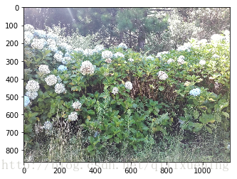
如上面两图所示，入侵物种特征为：似球状偏白的花和较宽厚的叶。

另外还可以注意到图像像素较多，而且测试集中有一张图的宽高比例是反的，因此有必要对图像的大小进行变换，使之适合现有的CNN算法。

我们可以使用scikit-image的tranform方法对图像进行变换，这样得到的图像的像素值会在 0 到 1 之间，同时还利用np.random.permutation()对图像的顺序shuffle一下，避免未知原始数据分布造成的人为影响。

x = np.empty(shape=(n_tr, 224, 224, 3))
y = np.empty(n_tr)
labels = train_labels.invasive.values

for k,v in enumerate(np.random.permutation(n_tr)):
    path = '{0}{1}.jpg'.format(trainpath, v+1)
    tr_im = io.imread(path)
    x[k] = transform.resize(tr_im, output_shape=(224, 224, 3))
    y[k] = labels[v]

x = x.astype('float32')  # elements in x are between 0 and 1 inclusively.

当数据变换完成后，可以将其保存起来，这样在以后的调用中会方便、快捷很多，尤其是在数据量较大的时候，更应该如此。

# 保存为h5文件
f = h5py.File('E:\\kaggle\invasive_species\\ndarray_train.h5','w')
f['x']=x
f['y']=y
f.close()

在读取数据的时候，注意末尾的[:] 不能省略。

# 读取h5文件
f = h5py.File('E:\\kaggle\invasive_species\\ndarray_train.h5','r')
x = f['x'][:]  # f.keys()可以查看所有的主键
y = f['y'][:]
f.close()

接下来可以直接利用scikit-learn的train_test_split来划分训练集、验证集。

from sklearn.model_selection import train_test_split

x_train, x_val, y_train, y_val = train_test_split(x, y, test_size=0.2)
print(x_train.shape,y_train.shape,x_val.shape,y_val.shape, sep='\n')

(1836, 224, 224, 3)
(1836,)
(459, 224, 224, 3)
(459,)

数据预处理完成后，就可以开始构建CNN网络了。首先导入不包含全连接层的VGG16模型（第一次运行会自动下载模型所含的权重，函数默认直接从github下载，速度可能较慢）。

from keras.models import Sequential, Model
from keras import applications
from keras.layers import Dropout, Flatten, Dense
from keras.optimizers import SGD

img_shape = (224, 224, 3)

base_model = applications.VGG16(weights='imagenet', include_top=False, input_shape=img_shape)

Using TensorFlow backend.

接下来构建我们自己的全连接层，并设置卷积层权重系数不参与训练，并完成模型编译。

add_model = Sequential()
add_model.add(Flatten(input_shape=base_model.output_shape[1:]))
add_model.add(Dense(256, activation='relu'))
add_model.add(Dense(1, activation='sigmoid'))

model = Model(inputs=base_model.input, outputs=add_model(base_model.output))

for layer in model.layers[:-1]:
    layer.trainable = False

model.compile(loss='binary_crossentropy', optimizer=SGD(lr=1e-4, momentum=0.9), metrics=['accuracy'])

可以直接查看我们建立的CNN模型的具体结构如下：

model.summary()

_________________________________________________________________
Layer (type)                 Output Shape              Param #   
=================================================================
input_1 (InputLayer)         (None, 224, 224, 3)       0         
_________________________________________________________________
block1_conv1 (Conv2D)        (None, 224, 224, 64)      1792      
_________________________________________________________________
block1_conv2 (Conv2D)        (None, 224, 224, 64)      36928     
_________________________________________________________________
block1_pool (MaxPooling2D)   (None, 112, 112, 64)      0         
_________________________________________________________________
block2_conv1 (Conv2D)        (None, 112, 112, 128)     73856     
_________________________________________________________________
block2_conv2 (Conv2D)        (None, 112, 112, 128)     147584    
_________________________________________________________________
block2_pool (MaxPooling2D)   (None, 56, 56, 128)       0         
_________________________________________________________________
block3_conv1 (Conv2D)        (None, 56, 56, 256)       295168    
_________________________________________________________________
block3_conv2 (Conv2D)        (None, 56, 56, 256)       590080    
_________________________________________________________________
block3_conv3 (Conv2D)        (None, 56, 56, 256)       590080    
_________________________________________________________________
block3_pool (MaxPooling2D)   (None, 28, 28, 256)       0         
_________________________________________________________________
block4_conv1 (Conv2D)        (None, 28, 28, 512)       1180160   
_________________________________________________________________
block4_conv2 (Conv2D)        (None, 28, 28, 512)       2359808   
_________________________________________________________________
block4_conv3 (Conv2D)        (None, 28, 28, 512)       2359808   
_________________________________________________________________
block4_pool (MaxPooling2D)   (None, 14, 14, 512)       0         
_________________________________________________________________
block5_conv1 (Conv2D)        (None, 14, 14, 512)       2359808   
_________________________________________________________________
block5_conv2 (Conv2D)        (None, 14, 14, 512)       2359808   
_________________________________________________________________
block5_conv3 (Conv2D)        (None, 14, 14, 512)       2359808   
_________________________________________________________________
block5_pool (MaxPooling2D)   (None, 7, 7, 512)         0         
_________________________________________________________________
sequential_1 (Sequential)    (None, 1)                 6423041   
=================================================================
Total params: 21,137,729
Trainable params: 6,423,041
Non-trainable params: 14,714,688
_________________________________________________________________

接下来是比较重要的部分，由于我们的数据量不够大，若直接重复训练可能性能提升并不好，因而需要采用ImageDataGenerator进行实时数据提升，它通过对所给的数据进行缩放、平移、剪切、翻转、旋转等操作产生新的图像，也能对输入图像进行去中心化、标准化等操作。此处需要对数据去中心化，否则后续的训练过程会遭遇梯度消失，模型的准确率无法逐步有效提升。为了节省时间（笔记本性能太差），只迭代了2轮，此时在测试集上的准确率也达到了86%。

# epochs for demonstration purposes

from keras.preprocessing.image import ImageDataGenerator
from keras.callbacks import ModelCheckpoint

batch_size = 10
epochs = 2

train_datagen = ImageDataGenerator(featurewise_center=True, rotation_range=30, zoom_range=0.2, width_shift_range=0.1,
                                   height_shift_range=0.1, horizontal_flip=True, fill_mode='nearest')
val_datagen = ImageDataGenerator(featurewise_center=True)

train_datagen.fit(x_train)
val_datagen.fit(x_val)

train_datagenerator = train_datagen.flow(x_train, y_train, batch_size=batch_size)
validation_generator = val_datagen.flow(x_val, y_val, batch_size=batch_size)

history = model.fit_generator(
    train_datagenerator,
    steps_per_epoch=x_train.shape[0] // batch_size,
    epochs=epochs,
    validation_data=validation_generator,
    validation_steps=50,
    callbacks=[ModelCheckpoint('VGG16-transferlearning.model', monitor='val_acc', save_best_only=True)])

Epoch 1/2
183/183 [==============================] - 780s - loss: 0.5579 - acc: 0.7038 - val_loss: 0.4187 - val_acc: 0.8156
Epoch 2/2
183/183 [==============================] - 792s - loss: 0.4199 - acc: 0.7978 - val_loss: 0.3384 - val_acc: 0.8637

Predict the test set

接下来对测试集数据进行预测。需要注意的是，在预测时，需要让测试集的数据生成器与验证集的一致，因为验证集的去中心化是基于验证集本身的，所以测试集也应该以验证集的数据进行去中心化。

from skimage import io, transform

n_test = len(os.listdir(testpath))
xx = np.empty(shape=(n_test, 224, 224, 3))
xx = xx.astype('float32')

for i in range(n_test):
    path = '{0}{1}.jpg'.format(testpath, i+1)
    test_im = io.imread(path)
    xx[i] = transform.resize(test_im, output_shape=(224, 224, 3))

# 保存为h5文件
f = h5py.File('E:\\kaggle\invasive_species\\ndarray_test.h5','w')
f['x']=xx
f.close()

# 读取h5文件
f = h5py.File('E:\\kaggle\invasive_species\\ndarray_test.h5','r')
x_test = f['x'][:]  # f.keys()可以查看所有的主键
f.close()
test_generator = val_datagen.flow(x_test, batch_size=1, shuffle=False)

result = model.predict_generator(test_generator, n_test)

然后，可以将输出的[0,1]的概率转化为0，1的标记，并写入csv文件。

result[result>0.5] = 1
result[result!=1] = 0
result[0]

array([ 1.], dtype=float32)

df = pd.read_csv('E:\\kaggle\invasive_species\\sample_submission.csv')
df.invasive = result.flatten()
df.head()

	name	invasive
0	1	1.0
1	2	0.0
2	3	0.0
3	4	0.0
4	5	1.0

df.to_csv('E:\\kaggle\invasive_species\\demo_submission.csv', index=False)

将其提交到kaggle上，得到测试集的Public LB为84%左右，表明模型并未出现过拟合。

基于此，我们可以尝试更多的数据处理手法，模型超参数调整，不同CNN模型比较、集成，并利用交叉验证做进一步改进。