"""
Created on Fri Oct 12 13:26:50 2018
@author: fengjuan
"""
import pandas as pd
import numpy as np
#导入matplotlib工具包的pyplot并简称为plt
import matplotlib.pyplot as plt
df_train=pd.read_csv('Breast-Cancer-train.csv')
df_test=pd.read_csv('Breast-Cancer-test.csv')
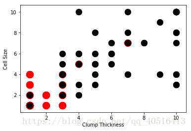
# 选取‘Clump Thickness’和 ‘Cell Size’作为特征值 ,构建测试集中的正负分类样本
df_test_negative=df_test.loc[df_test['Type']==0][['Clump Thickness','Cell Size']]
df_test_postive=df_test.loc[df_test['Type']==1][['Clump Thickness','Cell Size']]
# 绘制散点图 良性肿瘤样本点,标记为红色,恶性肿瘤样本点,标记为黑色
plt.scatter(df_test_negative['Clump Thickness'],df_test_negative['Cell Size'],marker='o',s=200,c='red')
plt.scatter(df_test_postive['Clump Thickness'],df_test_postive['Cell Size'],marker='o',s=150,c='black')
# 绘制x,y轴的说明
plt.xlabel('Clump Thickness')
plt.ylabel('Cell Size')
plt.show()#显示
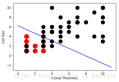
#利用numpy的random函数随机采样直线的截距和系数
# np.random.random([1])生成一个[0,1)之间的随机浮点数, np.random.random([2])生成两个[0,1)之间的随机浮点数
intercept=np.random.random([1])
coef=np.random.random([2])
lx=np.arange(0,12)
ly=(-intercept -lx*coef[0])/coef[1]
# 绘制一条随机直线
plt.plot(lx,ly,c='blue')
plt.scatter(df_test_negative['Clump Thickness'],df_test_negative['Cell Size'],marker='o',s=200,c='red')
plt.scatter(df_test_postive['Clump Thickness'],df_test_postive['Cell Size'],marker='o',s=150,c='black')
plt.xlabel('Clump Thickness')
plt.ylabel('Cell Size')
plt.show()
#导入sklearn中的逻辑斯蒂回归分类器
from sklearn.linear_model import LogisticRegression
lr = LogisticRegression()#注意这里的()不能丢
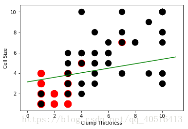
#使用前10条训练样本学习直线的系数和截距
lr.fit(df_train[['Clump Thickness', 'Cell Size']][:10], df_train['Type'][:10])
#输出测试准确率结果

结果为:
Testing accuracy is: 0.8685714285714285
print('Testing accuracy is:',lr.score(df_test[['Clump Thickness','Cell Size']],df_test['Type']))
intercept=lr.intercept_
coef=lr.coef_[0,:]
# 原本这个分类面应该是lx * coef[0]+ly*coef[1]+intercept=0,映射到2维平面上之后,应该是:
ly=(-intercept -lx*coef[0])/coef[1]
plt.plot(lx,ly,c='green')
plt.scatter(df_test_negative['Clump Thickness'],df_test_negative['Cell Size'],marker='o',s=200,c='red')
plt.scatter(df_test_postive['Clump Thickness'],df_test_postive['Cell Size'],marker='o',s=150,c='black')
plt.xlabel('Clump Thickness')
plt.ylabel('Cell Size')
plt.show()
#使用所有训练样本学习直线的系数和截距
lr=LogisticRegression()
lr.fit(df_train[['Clump Thickness', 'Cell Size']], df_train['Type'])
print('Testing accuracy(all samples) is:',lr.score(df_test[['Clump Thickness','Cell Size']],df_test['Type']))
结果是:Testing accuracy(all samples) is: 0.9371428571428572
intercept=lr.intercept_
coef=lr.coef_[0,:]
ly=(-intercept -lx*coef[0])/coef[1]
#1-5
plt.plot(lx,ly,c='blue')
plt.scatter(df_test_negative['Clump Thickness'],df_test_negative['Cell Size'],marker='o',s=200,c='red')#注意和前10的区别
plt.scatter(df_test_postive['Clump Thickness'],df_test_postive['Cell Size'],marker='o',s=150,c='black')
plt.xlabel('Clump Thickness')
plt.ylabel('Cell Size')
plt.show()