目录：
1. 半监督学习(Semi-supervised Learning SSL)
2. 完全图
 3. 标签传播算法的基本思路
 4. 标签传播算法
 5. 算法描述
 6. 标签传播算法的基本特点
 7. 代码实现

1. 半监督学习(Semi-supervised Learning SSL)

半监督学习是一种有监督学习和无监督学习想结合的一种方法，其主要思想是基于数据分布上的模型假设，利用少量的已标注数据进行指导并预测未标记数据的标记，并合并到标记数据集中去。

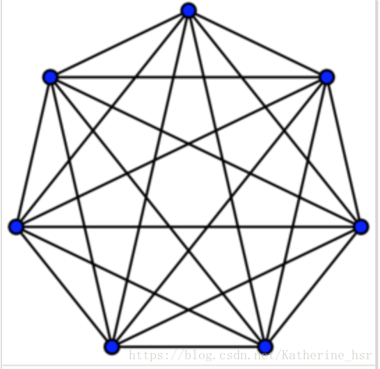
2. 完全图

在图论的数学领域，完全图是一个简单的无向图，其中每对不同的顶点之间都恰连有一条边相连。完整的有向图又是一个有向图，其中每对不同的顶点通过一对唯一的边缘（每个方向一个）连接。n个端点的完全图有n个端点以及n(n − 1) / 2条边，以Kn表示。它是(k − 1)-正则图。所有完全图都是它本身的团（clique）
这里写图片描述

3. 标签传播算法的基本思路

标签传播算法是基于图的半监督学习方法，基本思路是从已标记的节点的标签信息来预测未标记的节点的标签信息，利用样本间的关系，建立完全图模型。
每个节点标签按相似度传播给相邻节点，在节点传播的每一步，每个节点根据相邻节点的标签来更新自己的标签，与该节点相似度越大，其相邻节点对其标注的影响权值越大，相似节点的标签越趋于一致，其标签就越容易传播。在标签传播过程中，保持已标记的数据的标签不变，使其将标签传给未标注的数据。最终当迭代结束时，相似节点的概率分布趋于相似，可以划分到一类中。

4.标签传播算法

令 $(x_1, y_1)...(x_l, y_l)是已标注的数据，Y_L=\lbrace y_1, ... y_L \rbrace\in \lbrace1, ..., C\rbrace$ ,类别数C已知，且均存在于标签数据中。令 $(x_{l+1},y_{l+1})...(x_{l+u}, y_{l+u})为未标注数据，则Y_U=\lbrace y_{l+1}, ..., y_{l+u} \rbrace 是没有标签的，通常l<<u，也就是说有标签的数据的数量远远小于没有标签的数据的数量，让X= \lbrace{x_1, .., x_{l+u}} \rbrace\in R^D,则问题转换为从X和Y_L中去预测Y_U$ 。
我们想要相邻的数据点具有相同的标签，我们建立一个全连接图，让每一个样本点(有标签的和无标签的)都作为一个节点。用一下权重计算方式来设定两点i,j之间边的权重，所以两点间的距离 $d_{ij}$ 越小，权重 $w_{ij}$ 越大。
$w_{ij} = exp(-{\frac{d_{ij}}{\sigma^2}}) = exp(-{\frac{\sum^D_{d=1}(x_i^d - x_j^d)}{\sigma^2}})$
然后让每一个带有标签的节点通过边传播到所有的节点，权重大的边的节点更容易影响到相邻的节点。
我们定义一个(l+u)*(l+u)的概率传播矩阵T，让 $T_{ij}$ 为标签j传播到标签i的概率。
$T_{ij} = P(j\rightarrow i) = \frac{w_{ij}}{\sum_{k=1}^{l+u}w_{kj}}$
同时定义一个(l+u)*C的标签矩阵Y， $Y_{i,C}=\delta(y_i, C)$ ，它的第i行表示节点 $y_i$ 的标注概率，第C列代表类别。 $Y_{i,C}=1$ , 则说明节点 $y_i$ 的标签为C。通过概率传递，使其概率分布集中于给定类别，然后通过边的权重值来传递节点标签。

5. 算法描述

input：u个未标记数据和l个标记的数据及其标签
output：u个未标记数据的标签
第一步：初始化，利用权重公式来计算每条边的权重 $w_{ij}$ ，得到数据间的相似度
第二步：根据得到的权重 $w_{ij}$ , 计算节点j到i的传播概率 $T_{ij}$
第三步：定义一个(l+u)*C的矩阵
第四步：每个节点按传播概率把它周围节点传播的标注值按权重相加，并更新到自己的概率分布
第五步：限定已标注的数据，把已标注的数据的概率分布重新赋值为初始值，然后重复步骤四，直至收敛。

6. 标签传播算法的基本特点

(1) LPA是一种半监督学习方法，具有半监督学习算法的两个假设前提：1. 临近样本点具有相同的标签。根据该假设，分类时边界两侧尽可能避免选择较为密集的样本数据点，而是尽量选择稀疏数据，便于算法利用少了已标注数据指导大量的未标注数据。2. 相同流结构上的点能够拥有相同的标签。根据该假设，未标记的样本数据能够让数据空间变得更加密集，便于充分分析局部区域特征。
(2) LPA只需要利用少量的训练标签指导，利用未标注数据的内在结构，分布规律和临近数据的标记，即可预测和传播未标记数据的标签，然后合并到标记的数据集中。该算法操作简单，运算量小，适合大规模数据信息的挖掘和处理。
(3) LPA 可以通过相近节点之间的标签的传递来学习分类，所以它不受数据分布形状的局限。所以只要同一类的数据在空间分布上是相似的，那么不管数据分布是什么形状的，都能通过标签传播，把他们分到同一个类里。因此可以处理包括音频、视频、图像及文本的标注，检索及分类。

7. 代码实现

import time
import math
import numpy as np


# return k neighbors index
def navie_knn(dataSet, query, k):
    numSamples = dataSet.shape[0]

    ## step 1: calculate Euclidean distance
    diff = np.tile(query, (numSamples, 1)) - dataSet
    squaredDiff = diff ** 2
    squaredDist = np.sum(squaredDiff, axis=1)  # sum is performed by row

    ## step 2: sort the distance
    sortedDistIndices = np.argsort(squaredDist)
    if k > len(sortedDistIndices):
        k = len(sortedDistIndices)

    return sortedDistIndices[0:k]


# build a big graph (normalized weight matrix)
def buildGraph(MatX, kernel_type, rbf_sigma=None, knn_num_neighbors=None):
    num_samples = MatX.shape[0]
    affinity_matrix = np.zeros((num_samples, num_samples), np.float32)
    if kernel_type == 'rbf':
        if rbf_sigma == None:
            raise ValueError('You should input a sigma of rbf kernel!')
        for i in range(num_samples):
            row_sum = 0.0
            for j in range(num_samples):
                diff = MatX[i, :] - MatX[j, :]
                affinity_matrix[i][j] = np.exp(sum(diff ** 2) / (-2.0 * rbf_sigma ** 2))
                row_sum += affinity_matrix[i][j]
            affinity_matrix[i][:] /= row_sum
    elif kernel_type == 'knn':
        if knn_num_neighbors == None:
            raise ValueError('You should input a k of knn kernel!')
        for i in range(num_samples):
            k_neighbors = navie_knn(MatX, MatX[i, :], knn_num_neighbors)
            affinity_matrix[i][k_neighbors] = 1.0 / knn_num_neighbors
    else:
        raise NameError('Not support kernel type! You can use knn or rbf!')

    return affinity_matrix


# label propagation
def labelPropagation(Mat_Label, Mat_Unlabel, labels, kernel_type='rbf', rbf_sigma=1.5,
                     knn_num_neighbors=10, max_iter=500, tol=1e-3):
    # initialize
    num_label_samples = Mat_Label.shape[0]
    num_unlabel_samples = Mat_Unlabel.shape[0]
    num_samples = num_label_samples + num_unlabel_samples
    labels_list = np.unique(labels)
    num_classes = len(labels_list)

    MatX = np.vstack((Mat_Label, Mat_Unlabel))
    clamp_data_label = np.zeros((num_label_samples, num_classes), np.float32)
    for i in range(num_label_samples):
        clamp_data_label[i][labels[i]] = 1.0

    label_function = np.zeros((num_samples, num_classes), np.float32)
    label_function[0: num_label_samples] = clamp_data_label
    label_function[num_label_samples: num_samples] = -1

    # graph construction
    affinity_matrix = buildGraph(MatX, kernel_type, rbf_sigma, knn_num_neighbors)

    # start to propagation
    iter = 0;
    pre_label_function = np.zeros((num_samples, num_classes), np.float32)
    changed = np.abs(pre_label_function - label_function).sum()
    while iter < max_iter and changed > tol:
        if iter % 1 == 0:
            print("---> Iteration %d/%d, changed: %f" % (iter, max_iter, changed))
        pre_label_function = label_function
        iter += 1

        # propagation
        label_function = np.dot(affinity_matrix, label_function)

        # clamp
        label_function[0: num_label_samples] = clamp_data_label

        # check converge
        changed = np.abs(pre_label_function - label_function).sum()

    # get terminate label of unlabeled data
    unlabel_data_labels = np.zeros(num_unlabel_samples)
    for i in range(num_unlabel_samples):
        unlabel_data_labels[i] = np.argmax(label_function[i + num_label_samples])

    return unlabel_data_labels


# 测试代码
# show
def show(Mat_Label, labels, Mat_Unlabel, unlabel_data_labels):
    import matplotlib.pyplot as plt

    for i in range(Mat_Label.shape[0]):
        if int(labels[i]) == 0:
            plt.plot(Mat_Label[i, 0], Mat_Label[i, 1], 'Dr')
        elif int(labels[i]) == 1:
            plt.plot(Mat_Label[i, 0], Mat_Label[i, 1], 'Db')
        else:
            plt.plot(Mat_Label[i, 0], Mat_Label[i, 1], 'Dy')

    for i in range(Mat_Unlabel.shape[0]):
        if int(unlabel_data_labels[i]) == 0:
            plt.plot(Mat_Unlabel[i, 0], Mat_Unlabel[i, 1], 'or')
        elif int(unlabel_data_labels[i]) == 1:
            plt.plot(Mat_Unlabel[i, 0], Mat_Unlabel[i, 1], 'ob')
        else:
            plt.plot(Mat_Unlabel[i, 0], Mat_Unlabel[i, 1], 'oy')

    plt.xlabel('X1');
    plt.ylabel('X2')
    plt.xlim(0.0, 12.)
    plt.ylim(0.0, 12.)
    plt.show()


def loadCircleData(num_data):
    center = np.array([5.0, 5.0])
    radiu_inner = 2
    radiu_outer = 4
    num_inner = num_data // 3
    num_outer = num_data - num_inner

    data = []
    theta = 0.0
    for i in range(num_inner):
        pho = (theta % 360) * math.pi / 180
        tmp = np.zeros(2, np.float32)
        tmp[0] = radiu_inner * math.cos(pho) + np.random.rand(1) + center[0]
        tmp[1] = radiu_inner * math.sin(pho) + np.random.rand(1) + center[1]
        data.append(tmp)
        theta += 2

    theta = 0.0
    for i in range(num_outer):
        pho = (theta % 360) * math.pi / 180
        tmp = np.zeros(2, np.float32)
        tmp[0] = radiu_outer * math.cos(pho) + np.random.rand(1) + center[0]
        tmp[1] = radiu_outer * math.sin(pho) + np.random.rand(1) + center[1]
        data.append(tmp)
        theta += 1

    Mat_Label = np.zeros((2, 2), np.float32)
    Mat_Label[0] = center + np.array([-radiu_inner + 0.5, 0])
    Mat_Label[1] = center + np.array([-radiu_outer + 0.5, 0])
    labels = [0, 1]
    Mat_Unlabel = np.vstack(data)
    return Mat_Label, labels, Mat_Unlabel


def loadBandData(num_unlabel_samples):
    # Mat_Label = np.array([[5.0, 2.], [5.0, 8.0]])
    # labels = [0, 1]
    # Mat_Unlabel = np.array([[5.1, 2.], [5.0, 8.1]])

    Mat_Label = np.array([[5.0, 2.], [5.0, 8.0]])
    labels = [0, 1]
    num_dim = Mat_Label.shape[1]
    Mat_Unlabel = np.zeros((num_unlabel_samples, num_dim), np.float32)
    Mat_Unlabel[:num_unlabel_samples / 2, :] = (np.random.rand(num_unlabel_samples / 2, num_dim) - 0.5) * np.array(
        [3, 1]) + Mat_Label[0]
    Mat_Unlabel[num_unlabel_samples / 2: num_unlabel_samples, :] = (np.random.rand(num_unlabel_samples / 2,
                                                                                   num_dim) - 0.5) * np.array([3, 1]) + \
                                                                   Mat_Label[1]
    return Mat_Label, labels, Mat_Unlabel


# main function
if __name__ == "__main__":
    num_unlabel_samples = 800
    # Mat_Label, labels, Mat_Unlabel = loadBandData(num_unlabel_samples)
    Mat_Label, labels, Mat_Unlabel = loadCircleData(num_unlabel_samples)

    ## Notice: when use 'rbf' as our kernel, the choice of hyper parameter 'sigma' is very import! It should be
    ## chose according to your dataset, specific the distance of two data points. I think it should ensure that
    ## each point has about 10 knn or w_i,j is large enough. It also influence the speed of converge. So, may be
    ## 'knn' kernel is better!
    # unlabel_data_labels = labelPropagation(Mat_Label, Mat_Unlabel, labels, kernel_type = 'rbf', rbf_sigma = 0.2)
    unlabel_data_labels = labelPropagation(Mat_Label, Mat_Unlabel, labels, kernel_type='knn', knn_num_neighbors=10,
                                           max_iter=1)
    show(Mat_Label, labels, Mat_Unlabel, unlabel_data_labels)

当max_iter=1时
这里写图片描述
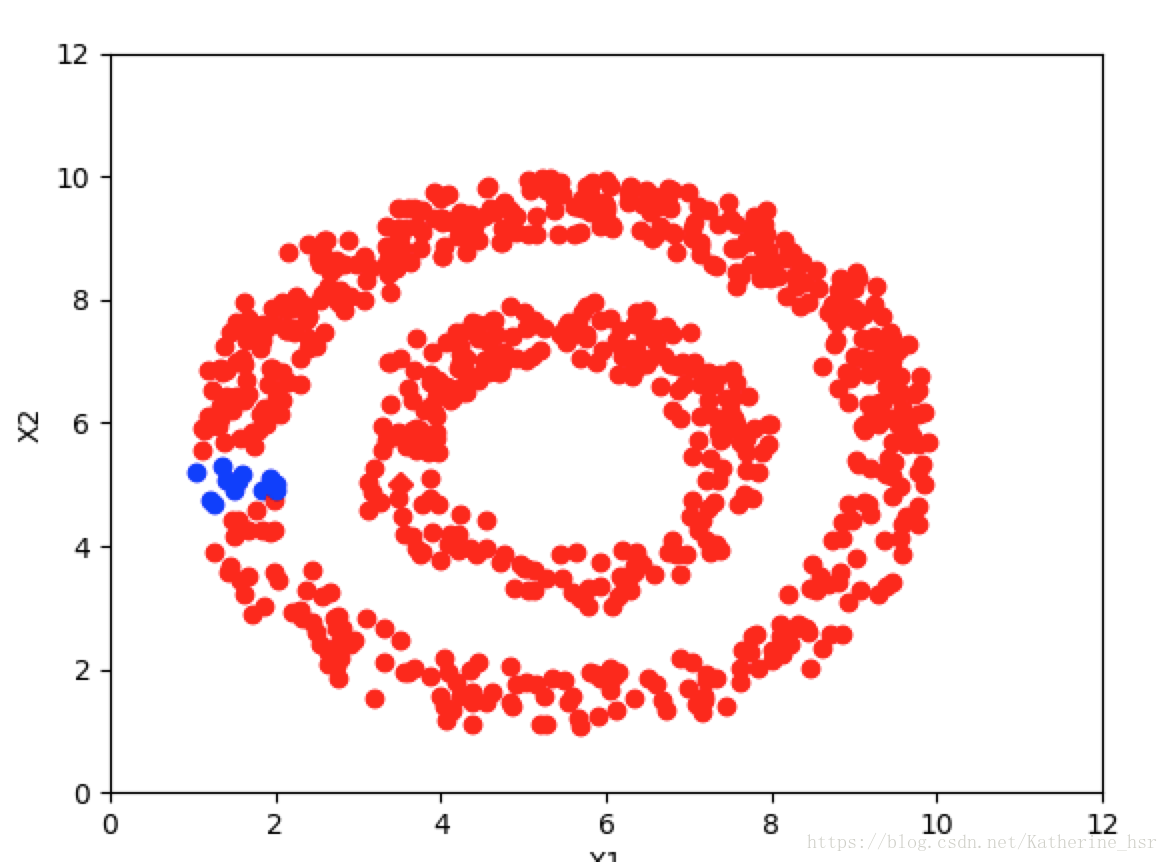
当max_iter=100时

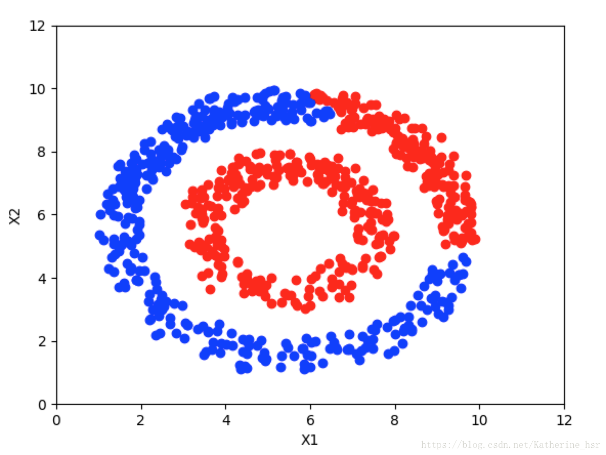
当max_iter=200时

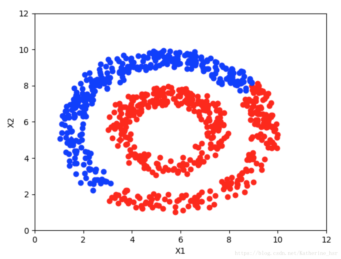
当max_iter=300时

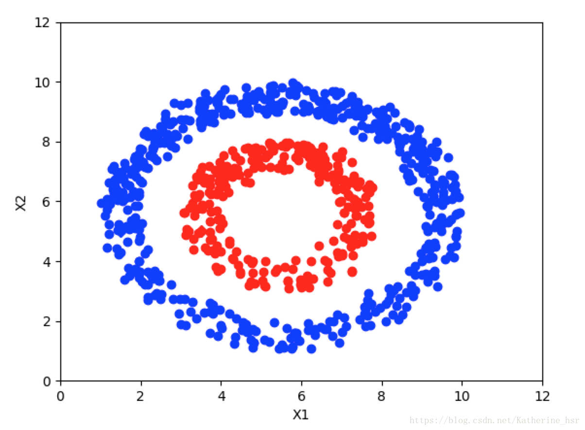
可以看出，随着迭代次数的增加逐步收敛。

标签传播算法(Label Propagation Algorithm)