本篇博客转自:NLTK学习之三:文本分类与构建基于分类的词性标注器
学习记录所用,如有侵权,立即删除。
一、有监督的分类
1、分类
分类时为给定输入选择正确的类标签的任务。比如判断一封Email是否是垃圾邮件,确定一篇新闻的主题。如果分类的时候需要人工标注的标签进行训练,则称为有监督的分类。
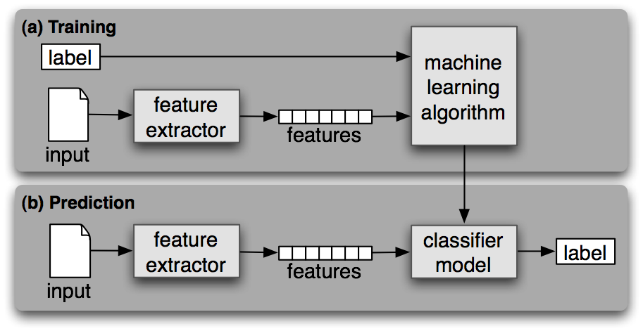
分类器需要决定选择什么样的特征,并对特征进行编码。
2、NLTK分类器
在NLTK中提供了NativeClassifier、DecisionTreeClassifier、MaxentClassifier三种类型的分类器。分类器都提供了类方法可以训练出一个分类器实例,有了这个实例,便能对新的样本进行分类预测,以及对其进行准确度评测。
train(train_set) 类方法,用于生成一个分类器实例
classify(feature) 实例方法,基于训练的模型对输入特征进行分类
show_most_informative_features() 实例方法,显示训练过程中最有效的特性统计
nltk.classify包的工具类提供了下列的方法辅助训练及优化过程
accuracy(classifier,test_set) 评估分类器在测试集上的准确度
apply_feature(func,data) 将特征函数func应用到data上,类似于map操作
3、文本分类示例
下面基于NLTK的movie_reviews语料库的正负向标注数据训练一个简单的分类器,用来预测评论的正负向。语料库被分为两类:pos与neg
代码先统计出最常用的2000个词,简单假设这些词的使用情况可以决定一篇评论的正负向情感。针对每个评论,特征提取器计算其在这2000个词上出现的情况,若出现则在特性中标记为True,否则标记为False。
代码示例:
import random
import nltk
from nltk.corpus import movie_reviews

docs = [(list(movie_reviews.words(fileid)), category)
        for category in movie_reviews.categories()   # 类别
        for fileid in movie_reviews.fileids(category)]  # 文件标识符

# 将数据随机打乱
random.shuffle(docs)

all_words = nltk.FreqDist(w.lower() for w in movie_reviews.words())
most_common_word = [word for (word, _) in all_words.most_common(2000)]


def doc_feature(doc):
    doc_words = set(doc)
    feature = {}
    for word in most_common_word:
        feature[word] = (word in doc_words)
    return feature

train_set = nltk.apply_features(doc_feature, docs[:100])
test_set = nltk.apply_features(doc_feature, docs[100:])

classifier = nltk.NaiveBayesClassifier.train(train_set)
print(nltk.classify.accuracy(classifier, test_set))
classifier.show_most_informative_features()
运行结果:
0.716842105263158
Most Informative Features
memorable = True pos : neg = 6.9 : 1.0
american = True pos : neg = 6.9 : 1.0
solid = True pos : neg = 6.9 : 1.0
supposed = True neg : pos = 6.3 : 1.0
local = True pos : neg = 6.1 : 1.0
looks = True neg : pos = 5.8 : 1.0
charm = True pos : neg = 5.3 : 1.0
oscar = True pos : neg = 5.3 : 1.0
famous = True pos : neg = 5.3 : 1.0
modern = True pos : neg = 5.3 : 1.0
4、基于上下文的词性标注器
N-gram Tagger的主要思想是基于词的词性的历史出现次数进行推测。接下来的介绍的是基于分类器的词性标注器,它借助于词本身,词的上下文,标注信息的上下文等特征来训练一个词性分类器,从而实现词性标注。
示例代码:
import nltk
from nltk.corpus import brown


def pos_feature_use_hist(sentence, i , history):
    features = {
        'suffix-1': sentence[i][-1:],
        'suffix-2': sentence[i][-2:],
        'suffix-3': sentence[i][-3:],
        'pre-word': 'START',
        'prev-tag': 'START'
    }
    if i > 0:
        features['pre-word'] = sentence[i - 1]
        features['prev-tag'] = history[i - 1]
    return features


class ContextPosTagger(nltk.TaggerI):
    def __init__(self, train):
        train_set = []
        for tagged_sent in train:
            untagged_sent = nltk.tag.untag(tagged_sent)
            history = []
            for i, (word, tag) in enumerate(tagged_sent):
                features = pos_feature_use_hist(untagged_sent, i, history)
                train_set.append((features, tag))
                history.append(tag)
        print(train_set[:10])
        self.classifier = nltk.NaiveBayesClassifier.train(train_set)

    def tag(self, sent):
        history = []
        for i, word in enumerate(sent):
            features = pos_feature_use_hist(sent, i, history)
            tag = self.classifier.classify(features)
            history.append(tag)
        return zip(sent, history)

tagged_sents = brown.tagged_sents(categories='news')
size = int(len(tagged_sents) * 0.8)
train_sets, test_sets = tagged_sents[0: size], tagged_sents[size:]

tagger = ContextPosTagger(train_sets)
tagger.classifier.show_most_informative_features()

print(tagger.evaluate(test_sets))
运行结果:
[({'suffix-1': 'e', 'suffix-2': 'he', 'suffix-3': 'The', 'pre-word': 'START', 'prev-tag': 'START'}, 'AT'), ({'suffix-1': 'n', 'suffix-2': 'on', 'suffix-3': 'ton', 'pre-word': 'The', 'prev-tag': 'AT'}, 'NP-TL'), ({'suffix-1': 'y', 'suffix-2': 'ty', 'suffix-3': 'nty', 'pre-word': 'Fulton', 'prev-tag': 'NP-TL'}, 'NN-TL'), ({'suffix-1': 'd', 'suffix-2': 'nd', 'suffix-3': 'and', 'pre-word': 'County', 'prev-tag': 'NN-TL'}, 'JJ-TL'), ({'suffix-1': 'y', 'suffix-2': 'ry', 'suffix-3': 'ury', 'pre-word': 'Grand', 'prev-tag': 'JJ-TL'}, 'NN-TL'), ({'suffix-1': 'd', 'suffix-2': 'id', 'suffix-3': 'aid', 'pre-word': 'Jury', 'prev-tag': 'NN-TL'}, 'VBD'), ({'suffix-1': 'y', 'suffix-2': 'ay', 'suffix-3': 'day', 'pre-word': 'said', 'prev-tag': 'VBD'}, 'NR'), ({'suffix-1': 'n', 'suffix-2': 'an', 'suffix-3': 'an', 'pre-word': 'Friday', 'prev-tag': 'NR'}, 'AT'), ({'suffix-1': 'n', 'suffix-2': 'on', 'suffix-3': 'ion', 'pre-word': 'an', 'prev-tag': 'AT'}, 'NN'), ({'suffix-1': 'f', 'suffix-2': 'of', 'suffix-3': 'of', 'pre-word': 'investigation', 'prev-tag': 'NN'}, 'IN')]
Most Informative Features
suffix-1 = '.' . : NN = 6459.2 : 1.0
suffix-2 = 'he' AT : NN = 2991.3 : 1.0
prev-tag = 'TO' VB : NN = 2891.2 : 1.0
suffix-2 = 'ho' WPS : NN = 2596.0 : 1.0
prev-tag = 'MD' BE : AT = 2582.0 : 1.0
prev-tag = 'HVZ' BEN : NN = 2005.9 : 1.0
suffix-2 = 'to' TO : JJ = 1822.0 : 1.0
suffix-2 = 'be' BE : NP = 1504.3 : 1.0
suffix-3 = 'hat' CS : NN = 1466.9 : 1.0
suffix-2 = 'es' NNS : IN = 1403.8 : 1.0
5、算法评估方法
对于分类算法在测试集上运行之后,数据会被分为下表的四类
分类为正 TP(真正例) FP(假正例)
分类为负 FN(假负例) TN(真负例)
准确度A:(TP+TN)/ALL 分类器正确分类的比例。
精确度P:TP/(TP+FP), 预测为正的样本中,有多少真的正样本
召回率R:TP/(TP+FN),测试集中的正样本,有多少被正确分类
F1评分:(2*P*R)/(P+R),R与P的调和平均数
6、对于多分类任务,可以使用混淆矩阵来分析错误分类的细分信息。混淆矩阵的元素m[i, j],表示正确的类别i,被预测为类别j的次数。
示例代码:
import nltk
gold = [1, 2, 3, 4]
test = [1, 3, 2, 4]
print(nltk.ConfusionMatrix(gold, test))
运行结果:
| 1 2 3 4 |
--+---------+
1 |<1>. . . |
2 | .<.>1 . |
3 | . 1<.>. |
4 | . . .<1>|
--+---------+
(row = reference; col = test)
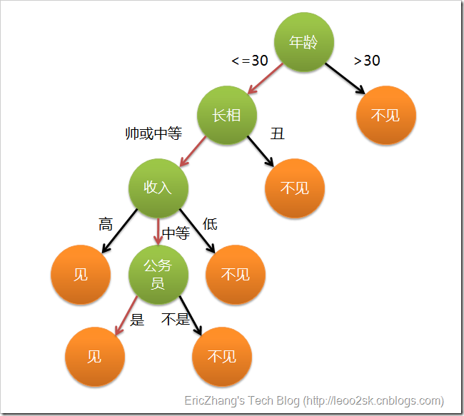
7、决策树(decision tree)分类器
决策树是一个树结构,其每个非叶节点表示一个特征属性上的测试,而每个叶节点存放一个类别。使用决策树进行决策的过程就是从根节点开始,测试待分类项中相应的特征属性,并按照其值选择输出分支,知道到达叶子节点,将叶子节点存放的类别作为决策结果。
8、朴素贝叶斯分类器
由条件概率和乘法法则:

对于贝叶斯分类器,假设某个样本集有n项特征(Feature),分别为F1、F2、...、Fn。现有m个类别(Category),分别为C1、C2、...、Cm。分类器就是计算出概率最大的那个分类,也就是求出下面算式的最大值:

由于P(F1F2...Fn)对于所有的类别都是相同的,可以省略,问题就变成了求P(F1F2...Fn)P(C)的最大值,朴素贝叶斯分类器则是更进一步,假设所有特征都相互独立,因此有

9、最大熵分类器
在信息论中,熵表示离散随机事件的出现概率。一个系统越是有序,信息熵就越低;反之,一个系统越是混乱,信息熵就越高。
9.1 熵
如果一个随机变量X的可能值X={X1,X2,...,Xk},其概率分布为P(X=xi)=pi(i=1,2,...,n),则随机变量X的熵定义为:

9.2条件熵
对于两个随机变量X,Y的联合分布,可以形成联合熵Joint Entropy,用H(X,Y)表示
在随机变量X发生的前提下,随机变量Y发生所新带来的熵定义为Y的条件熵,用H(Y|X)表示,用来衡量在已知随机变量X的条件下随机变量Y的不确定性,定义为:

9.3 相对熵
又称互熵,交叉熵,设p(x)、q(x)是X中取值的两个概率分布,则p对q的相对熵为:

9.4 互信息
两个随机变量X,Y的互信息定义为X,Y的联合分布和各自独立分布乘积的相对熵,用I(X,Y)表示

9.5 最大熵模型
最大熵模型的本质,即为已知X,计算Y的概率,且尽可能让Y的概率最大(实践中,X可能是某单词的上下文信息,Y是该单词翻译成me,I,us,we的各自概率),从而根据各自信息,尽可能最准确的推测未知信息。模型表示为:

求解最大熵参数的算法有GIS,IIS,MEGAM,TADM,可以在nltk.classify,maxent类中找到实现。