(未完)
5.1 Classification 分类学习
Classification 分类问题,定性输出是分类,或者说是离散变量预测。
Regression 回归问题,定量输出是回归,或者说是连续变量预测。
"""
Please note, this code is only for python 3+. If you are using python 2+, please modify the code accordingly.
"""
from __future__ import print_function #强制使用python3的语法,不管你环境中的python是什么版本
import tensorflow as tf
from tensorflow.examples.tutorials.mnist import input_data #导入mnist库
# number 1 to 10 data
mnist = input_data.read_data_sets('MNIST_data', one_hot=True) #如果没有mnist数据就进行下载;使用one_hot编码
def add_layer(inputs, in_size, out_size, activation_function=None,): #神经网络函数
# add one more layer and return the output of this layer
Weights = tf.Variable(tf.random_normal([in_size, out_size]))
biases = tf.Variable(tf.zeros([1, out_size]) + 0.1,)
Wx_plus_b = tf.matmul(inputs, Weights) + biases
if activation_function is None:
outputs = Wx_plus_b
else:
outputs = activation_function(Wx_plus_b)
return outputs
def compute_accuracy(v_xs, v_ys): #计算精度函数
global prediction #在函数里定义全局变量
y_pre = sess.run(prediction, feed_dict={xs: v_xs})
correct_prediction = tf.equal(tf.argmax(y_pre,1), tf.argmax(v_ys,1)) #函数tf.equal(x,y,name=None)对比x与y矩阵/向量中相等的元素,相等的返回True,不相等返回False,返回的矩阵/向量的维度与x相同;tf.argmax()返回最大值对应的下标(1表示每一列中的,0表示每一行)
accuracy = tf.reduce_mean(tf.cast(correct_prediction, tf.float32)) #tf.cast()类型转换函数,将correct_prediction转换成float32类型,并对correct_prediction求平均值得到arruracy
result = sess.run(accuracy, feed_dict={xs: v_xs, ys: v_ys})
return result
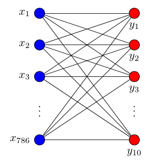
# define placeholder for inputs to network
xs = tf.placeholder(tf.float32, [None, 784]) #输入为N个图片,每个图片由28x28=784个像素点组成
ys = tf.placeholder(tf.float32, [None, 10]) #输出N个数据,每张图片识别一个数字0-9共10种
# add output layer
prediction = add_layer(xs, 784, 10, activation_function=tf.nn.softmax) #输入784,输出10,激励函数使用softmax
# the error between prediction and real data
cross_entropy = tf.reduce_mean(-tf.reduce_sum(ys * tf.log(prediction),
reduction_indices=[1])) #loss函数(即最优化目标函数)选用交叉熵函数。交叉熵用来衡量预测值和真实值的相似程度,如果完全相同,它们的交叉熵等于零。
train_step = tf.train.GradientDescentOptimizer(0.5).minimize(cross_entropy) #梯度下降法
sess = tf.Session()
# important step
# tf.initialize_all_variables() no long valid from
# 2017-03-02 if using tensorflow >= 0.12
if int((tf.__version__).split('.')[1]) < 12 and int((tf.__version__).split('.')[0]) < 1:
init = tf.initialize_all_variables()
else:
init = tf.global_variables_initializer()
sess.run(init)
#sess.run(tf.global_variables_initializer()) #初始化模型的参数
for i in range(1000): #训练
batch_xs, batch_ys = mnist.train.next_batch(100) #每次采用100个图片进行训练,避免年数据过大,训练太慢
sess.run(train_step, feed_dict={xs: batch_xs, ys: batch_ys})
if i % 50 == 0:
print(compute_accuracy(
mnist.test.images, mnist.test.labels)) #测试集,images是输入,labels是输出
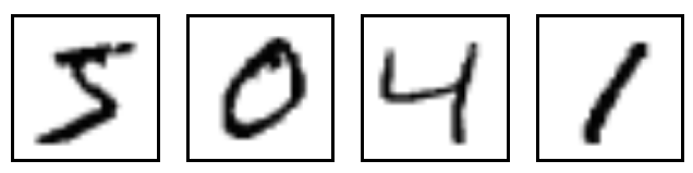
关于MNIST库:
MNIST库是手写数字库,含55000张训练图片,每张图片的分辨率是28×28。
from tensorflow.examples.tutorials.mnist import input_data
mnist = input_data.read_data_sets("MNIST_data/", one_hot=True)

print(mnist.train.images.shape) #训练
print(mnist.train.labels.shape)
print(mnist.validation.images.shape) #校验
print(mnist.validation.labels.shape)
print(mnist.test.images.shape) #测试
print(mnist.test.labels.shape)
softmax激励函数
5.2 什么是过拟合 overfitting
过拟合 = 自负 (学习的太好了,实际应用却不适用)
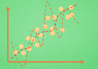
对于一个分类问题,通过学习与训练神经网络得出一条直线/曲线,来将两种颜色的原点进行区分,学习得到的曲线的误差可能会很大也可能会很小。
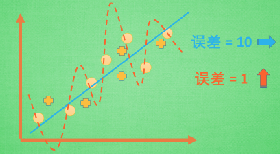
当然了,误差小只能说明,对于已经给定的训练集效果会非常好,但是如果在实际应用当中或者给定另外一组测试集,它的效果可能反而会变得很差。
解决办法
解决办法无非就是两种
第一种就是增加数据集,给神经网络更多的数据来让他进行学习训练,得到更加精确的分类曲线。大部分的过拟合问题都是由于我们的数据量不够,果我们有成千上万的数据,红线也会慢慢被拉直,变得没那么扭曲。
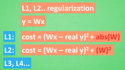
第二种就是使用一些防止过拟合的方法,利用L1,L2·····正则化(regularization),Dropout方法等。
我们简化机器学习的关键公式为 y=Wx ,W为机器需要学习到的各种参数。在过拟合中,W 的值往往变化得特别大或特别小。为了不让W变化太大,我们在计算误差上做些手脚。原始的cost = 预测值-真实值的平方。如果 W 变得太大,我们就让 cost 也跟着变大,变成一种惩罚机制。所以我们把 W 自己考虑进来。这里 abs 是绝对值。
其他的L2,L3,L4也都是换成了平方立方和4次方等等。用这些方法,我们就能保证让学出来的线条不会过于扭曲。
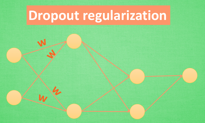
Dropout方法,专门用在神经网络上的一种方法,在训练开始前,随机删掉隐藏层中的一部分神经元,形成一个不完整的神经网络进行训练一次,第二次训练开始前又恢复成了一个完整的神经网络,然后再随机删除一部分神经元,再进行不完整的一次训练。这样做的目的就是每一次预测结果都不会依赖于其中某部分特定的神经元。像L1,L2正规化一样,过度依赖的 W,也就是训练参数的数值会很大,L1,L2会惩罚这些大的参数。Dropout 的做法是从根本上让神经网络没机会过度依赖。
5.3 Dropout 解决 overfitting
from __future__ import print_function
import tensorflow as tf
from sklearn.datasets import load_digits
from sklearn.model_selection import train_test_split
from sklearn.preprocessing import LabelBinarizer

# load data
digits = load_digits()
X = digits.data
y = digits.target
y = LabelBinarizer().fit_transform(y)
X_train, X_test, y_train, y_test = train_test_split(X, y, test_size=.3)


def add_layer(inputs, in_size, out_size, layer_name, activation_function=None, ):
    # add one more layer and return the output of this layer
    Weights = tf.Variable(tf.random_normal([in_size, out_size]))
    biases = tf.Variable(tf.zeros([1, out_size]) + 0.1, )
    Wx_plus_b = tf.matmul(inputs, Weights) + biases
    # here to dropout
    Wx_plus_b = tf.nn.dropout(Wx_plus_b, keep_prob)
    if activation_function is None:
        outputs = Wx_plus_b
    else:
        outputs = activation_function(Wx_plus_b, )
    tf.summary.histogram(layer_name + '/outputs', outputs)
    return outputs


# define placeholder for inputs to network
keep_prob = tf.placeholder(tf.float32)
xs = tf.placeholder(tf.float32, [None, 64])  # 8x8
ys = tf.placeholder(tf.float32, [None, 10])

# add output layer
l1 = add_layer(xs, 64, 50, 'l1', activation_function=tf.nn.tanh)
prediction = add_layer(l1, 50, 10, 'l2', activation_function=tf.nn.softmax)

# the loss between prediction and real data
cross_entropy = tf.reduce_mean(-tf.reduce_sum(ys * tf.log(prediction),
                                              reduction_indices=[1]))  # loss
tf.summary.scalar('loss', cross_entropy)
train_step = tf.train.GradientDescentOptimizer(0.5).minimize(cross_entropy)

sess = tf.Session()
merged = tf.summary.merge_all()
# summary writer goes in here
train_writer = tf.summary.FileWriter("logs/train", sess.graph)
test_writer = tf.summary.FileWriter("logs/test", sess.graph)

# tf.initialize_all_variables() no long valid from
# 2017-03-02 if using tensorflow >= 0.12
if int((tf.__version__).split('.')[1]) < 12 and int((tf.__version__).split('.')[0]) < 1:
    init = tf.initialize_all_variables()
else:
    init = tf.global_variables_initializer()
sess.run(init)
for i in range(500):
    # here to determine the keeping probability
    sess.run(train_step, feed_dict={xs: X_train, ys: y_train, keep_prob: 0.5})
    if i % 50 == 0:
        # record loss
        train_result = sess.run(merged, feed_dict={xs: X_train, ys: y_train, keep_prob: 1})
        test_result = sess.run(merged, feed_dict={xs: X_test, ys: y_test, keep_prob: 1})
        train_writer.add_summary(train_result, i)
        test_writer.add_summary(test_result, i)