在我以前的一篇文章(https://blog.datadive.net/interpreting-random-forests/)中,我讨论了随机森林如何变成一个「白箱子」,这样每次预测就能被分解为各项特征的贡献和,即预测=偏差+特征 1 贡献+ ... +特征 n 贡献。
我的一些代码包正在做相关工作,然而,大多数随机森林算法包(包括 scikit-learn)并没有给出预测过程的树路径。因此 sklearn 的应用需要一个补丁来展现这些路径。幸运的是,从 0.17 版本的 scikit-learn 开始,在 api 中有两个新增功能,这使得这个过程相对而言比较容易理解 : 获取用于预测的所有叶子节点的 id ,并存储所有决策树的所有节点中间值,而不仅仅只存叶子节点的。通过这些,我们可以提取每个单独预测的树路径,并通过检查路径来分解这些预测过程。
闲话少说,代码托管在 github(https://github.com/andosa/treeinterpreter) ,你也可以通过 pip install treeinterpreter 来获取。
注意:这需要 0.17 版本的 scikit-learn ,你可以通过访问 http://scikit-learn.org/stable/install.html#install-bleeding-edge 这个网址来进行安装。
使用 treeinterpreter 分解随机森林
首先我们将使用一个简单的数据集,来训练随机森林模型。在对测试集的进行预测的同时我们将对预测值进行分解。
from treeinterpreter import treeinterpreter as ti
from sklearn.tree import DecisionTreeRegressor
from sklearn.ensemble import RandomForestRegressor
import numpy as np

from sklearn.datasets import load_boston
boston = load_boston()
rf = RandomForestRegressor()
rf.fit(boston.data[:300], boston.target[:300])
从模型中任意选择两个产生不同价格预测的数据点
instances = boston.data[[300, 309]]
print "Instance 0 prediction:", rf.predict(instances[0])
print "Instance 1 prediction:", rf.predict(instances[1])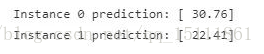
对于这两个数据点,随机森林给出了差异很大的预测值。为什么呢?我们现在可以将预测值分解成偏差项(就是训练集的均值)和单个特征贡献值,以便于观察究竟哪些特征项造成了差异,差异程度有多大。
我们可以简单地使用 treeinterpreter 中 predict 方法,向其传入模型和数据作为参数。
prediction, bias, contributions = ti.predict(rf, instances)将表格打印出来
for i in range(len(instances)):
   print "Instance", i
   print "Bias (trainset mean)", biases[i]
   print "Feature contributions:"
   for c, feature in sorted(zip(contributions[i],
                                boston.feature_names),
                            key=lambda x: -abs(x[0])):
       print feature, round(c, 2)
   print "-"*20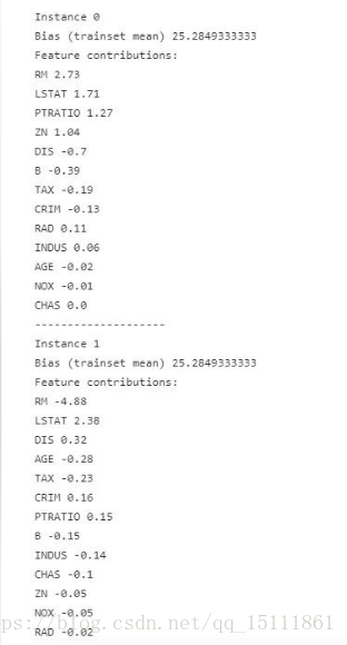
各个特征的贡献度按照绝对值从大到小排序。我们观察到第一个样本的预测结果较高,正贡献值主要来自 RM 、LSTAT 和 PTRATIO。第二个样本的预测值则低得多,因为 RM 实际上对预测值有着很大的负影响,而且这个影响并没有被其他正效应所补偿,因此低于数据集的均值。
但是这个分解真的是对的么?这很容易检查:偏差和各个特征的贡献值加起来需要等于预测值。
print prediction
print biases + np.sum(contributions, axis=1)
[ 30.76 22.41]
[ 30.76 22.41]
请注意,在把贡献值相加时,我们需要对浮点数进行处理,所以经过四舍五入处理后的值可能略有不同。
比较两个数据集
在对比两个数据集时,这个方法将会很有用。例如
理解导致两个预测值不同的真实原因,究竟是什么导致了房价在两个社区的预测值不同 。
调试模型或者数据,理解为什么新数据集的平均预测值与旧数据集所得到的结果不同。
还是上面这个例子,我们把房价数据的测试集再一分为二,分别计算它们的平均预测价值。
ds1 = boston.data[300:400]
ds2 = boston.data[400:]

print np.mean(rf.predict(ds1))
print np.mean(rf.predict(ds2))
22.1912
18.4773584906
我们发现两个数据集的平均预测值完全不同。现在我们就来看看导致差异的因素:究竟哪些特征造成了差异,差异程度有多大。
prediction1, bias1, contributions1 = ti.predict(rf, ds1)
prediction2, bias2, contributions2 = ti.predict(rf, ds2)
我们再来计算每一维特征的平均贡献程度。
totalc1 = np.mean(contributions1, axis=0)
totalc2 = np.mean(contributions2, axis=0)
因为两个测试集的偏差都是相同的(因为它们来自同一个训练集),那么两者平均预测值的不同主要是因为特征的贡献值不同。换句话说, 特征贡献差异的总和应该与平均预测的差异相等,这个很容易进行验证。
print np.sum(totalc1 - totalc2)
print np.mean(prediction1) - np.mean(prediction2)

3.71384150943
3.71384150943
最后,我们把每一维特征贡献的差异之和打印出来,这正好就是平均预测值的差异。
for c, feature in sorted(zip(totalc1 - totalc2,
                            boston.feature_names), reverse=True):
   print feature, round(c, 2)
分类树和森林
同样的方法也能用于分类树,查看特征对某个类别的预测概率值的影响力。
我们可以使用 iris 数据集做演示。
from sklearn.ensemble import RandomForestClassifier
from sklearn.datasets import load_iris
iris = load_iris()

rf = RandomForestClassifier(max_depth = 4)
idx = range(len(iris.target))
np.random.shuffle(idx)

rf.fit(iris.data[idx][:100], iris.target[idx][:100])
对一个独立样本做预测。
instance = iris.data[idx][100:101]
print rf.predict_proba(instance)
拆分每一维特征的贡献值
prediction, bias, contributions = ti.predict(rf, instance)
print "Prediction", prediction
print "Bias (trainset prior)", bias
print "Feature contributions:"
for c, feature in zip(contributions[0],
                            iris.feature_names):
   print feature, c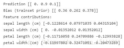
我们可以看到,对第二类预测能力最强的特征是花瓣长度和宽度,它们极大提高了预测的概率值。
总结
对随机森林预测值的理解其实是很简单的,与理解线性模型的难度相同。通过使用 treeinterpreter (pip install treeinterpreter),简单的几行代码就可以解决问题。
非常感谢阅读本文!
原文链接:
https://blog.datadive.net/random-forest-interpretation-with-scikit-learn