Introductory Guide – Factorization Machines & their application on huge datasets

Introduction

I still remember my first encounter with a Click prediction problem. Before this, I had been learning data science and I was feeling good about my progress. I had started to build my confidence in ML hackathons and I was determined to do well in several challenges.

In order to do well, I had even procured a machine with 16 GB RAM and i7 processor. But the first look at the dataset gave me jitters. The data when unzipped was over 50 GB – I had no clue how to predict a click on such a dataset. Thankfully Factorization machines came to my rescue.

Anyone who has worked on a Click Prediction problem or Recommendation systems would have faced a similar situation. Since the datasets are huge, doing predictions for these datasets becomes challenging with limited computation resources.

However, in most cases these datasets are sparse (only a few variables for each training example are non zero) due to which there are several features which are not important for prediction, this is where factorization helps to extract the most important latent or hidden features from the existing raw ones.

Factorization helps in representing approximately the same relationship between the target and predictors using a lower dimension dense matrix. In this article, I discuss Factorization Machines(FM) and Field Aware Factorization Machines(FFM) which allows us to take advantage of factorization in a regression/classification problem with an implementation using python.

Intuition behind Factorization
How Factorization Machines trump Polynomial and linear models?
Field Aware Factorization Machines (FFMs)
Implementation using xLearn Library in Python

Intuition behind Factorization

To get an intuitive understanding of matrix factorization, Let us consider an example: Suppose we have a user-movie matrix of ratings(1-5) where each value of the matrix represents rating (1-5) given by the user to the movie.

	Star Wars I	Inception	Godfather	The Notebook
U1	5	3	–	1
U2	4	–	–	1
U3	1	1	–	5
U4	1	–	–	4
U5	–	1	5	4

We observe from the table above that some of the ratings are missing and we would like to devise a method to predict these missing ratings. The intuition behind using matrix factorization to solve this problem is that there should be some latent features that determines how a user rates a movie. For example – users A and B would rate an Al Pacino movie highly if both of them are fans of actor Al Pacino, here a preference towards a particular actor would be a hidden feature since we are not explicitly including it in the rating matrix.

Suppose we want to compute K hidden or latent features. Our task is to find out the matrices P(U x K) and Q(D x K) (U – Users, D – Movies) such that P x Q^T approximates R which is the rating matrix. 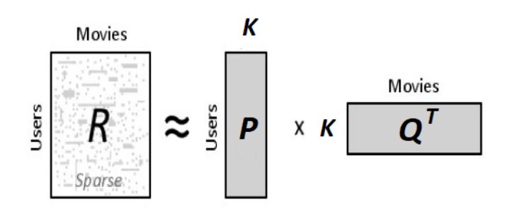Now, each row of P will represent strength of association between user and the feature while each row of Q represents the same strength w.r.t. the movie. To get the rating of a movie d_j rated by user u_i, we can calculate the dot product of 2 vectors corresponding to u_i and d_j All we need to do now is calculate P and Q matrices. We use gradient descent algorithm for doing this. The objective is to minimize the squared error between the actual rating and the one estimated by P and Q. The squared error is given by the following equation.

Now, we need to define an update rule for p_ik and q_kj. The update rule in gradient descent is defined by the gradient of the error to be minimized.

Having obtained the gradient, we can now formulate the update rules for both p_ik and q_kj

Here, α is the learning rate which can control the size of updates. Using the above update rules, we can then iteratively perform the operation until the error converges to its minimum. We can check the overall error as calculated using the following equation and determine when we should stop the process.

The above solution is simple and often leads to overfitting where the existing ratings are predicted accurately but it does not generalize well on unseen data. To tackle this we can introduce a regularization parameter β which will control the user-feature and movie-feature vectors in P and Q respectively and give a good approximation for the ratings.

For anyone interested in python implementation and exact details of the same may go to this link. Once we have calculated P and Q using the above methodology, we get the approximate rating matrix as:

	Star Wars I	Inception	Godfather	The Notebook
U1	4.97	2.98	2.18	0.98
U2	3.97	2.4	1.97	0.99
U3	1.02	0.93	5.32	4.93
U4	1.00	0.85	4.59	3.93
U5	1.36	1.07	4.89	4.12

Notice how we are able to regenerate the existing ratings, moreover we are now able to get a fair approximation to the unknown rating values.

How Factorization Machines trump Polynomial and linear models?

Let us consider a couple of training examples from a click prediction dataset. The dataset is click through related sports news website (publisher) and sports gear firms (advertiser).

Clicked	Publisher (P)	Advertiser (A)	Gender (G)
Yes	ESPN	Nike	Male
No	NBC	Adidas	Male

When we talk about FMs or FFMs, each column (Publisher, Advertiser…) in the dataset would be referred to as a field and each value (ESPN, Nike….) would be referred to as a feature.

A linear or a logistic modeling technique is great and does well in a variety of problems but the drawback is that the model only learns the effect of all variables or features individually rather than in combination.

$\phi _{LM} = w_{0} + w_{ESPN}x_{ESPN} + w_{Nike}x_{Nike} + w_{Adidas}x_{Adidas} + w_{NBC}x_{NBC} + w_{Male}x_{Male}$

Where w₀, w_ESPN etc. represent the parameters and x_ESPN, x_Nikerepresent the individual features in the dataset. By minimizing the log-loss for the above function we get logistic regression. One way to capture the feature interactions is a polynomial function that learns a separate parameter for the product of each pair of features treating each product as a separate variable.

$\phi _{Poly2} = w_{0} + w_{ESPN}x_{ESPN} + w_{Nike}x_{Nike} + w_{Adidas}x_{Adidas} + w_{NBC}x_{NBC} + w_{Male}x_{Male}$

$+ w_{ESPN,Nike}x_{ESPN}x_{Nike} + w_{ESPN,Male}x_{ESPN}x_{Male} + .............$

This can also be referred to as Poly2 model as we are only considering combination of 2 features for a term.

The problem with this is that even for a medium sized dataset, we have a huge model that has terrible implications for both the amount of memory needed to store the model and the time it takes to train the model.
Secondly, for a sparse dataset this technique will not do well to learn all the weights or parameters reliably i.e. we will not have enough training examples for each pair of features in order for each weight to be reliable.

FM to the rescue

FM solves the problem of considering pairwise feature interactions. It allows us to train, based on reliable information (latent features) from every pairwise combination of features in the model. FM also allows us to do this in an efficient way both in terms of time and space complexity. It models pairwise feature interactions as the dot product of low dimensional vectors(length = k). This is illustrated with the following equation for a degree = 2 factorization machine: Each parameter in FMs (k=3) can be described as follows: Here, for each term we have calculated the dot product of the 2 latent factors of size 3 corresponding to the 2 features.

From a modeling perspective, this is powerful because each feature ends up transformed to a space where similar features are embedded near one another. In simple words, the dot product basically represents similarity of the hidden features and it is higher when the features are in the neighborhood.

The cosine function is 1 (maximum) when theta is 0 and decreases to -1 when theta is 180 degrees. It is clear that the similarity is maximum when theta approaches 0.

Another big advantage of FMs is that we are able to compute the term that models all pairwise interactions in linear time complexity using a simple mathematical manipulation to the above equation. If you want to have a look at the exact steps required for this, please refer to the original Factorization Machines research paper at this link.

Example: Demonstration of how FM is better than POLY2

Consider the following artificial Click Through Rate (CTR) data:

This is a dataset comprising of sports websites as publishers and sports gear brands as publishers. The ad appears as a popup and the user has an option of clicking (clicks)the ad or closing it (unclicks).

There is only one negative training data for the pair (ESPN, Adidas). For Poly2, a very negative weight w_ESPN,Adidas might be learned for this pair. For FMs, because the prediction of (ESPN, Adidas) is determined by w_ESPN·w_Adidas, and because w_ESPN and w_Adidas are also learned from other pairs of features as well (e.g., (ESPN, Nike), (NBC, Adidas)), the prediction may be more accurate.
Another example is that there is no training data for the pair (NBC, Gucci). For Poly2, the prediction on this pair is 0, but for FMs, because w_NBC and w_Gucci can be learned from other pairs, it is still possible to do meaningful prediction.

Field-Aware Factorization Machines

Clicked	Publisher (P)	Advertisor (A)	Gender (G)
Yes	ESPN	Nike	Male

In order to understand FFMs, we need to realize the meaning of field. Field is typically the broader category which contains a particular feature. In the above training example, the fields are Publisher (P), Advertiser (A) and Gender(G).

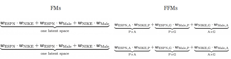
In FMs, every feature has only one latent vector v to learn the latent effect with any other features. Take ESPN as an example, w_ESPN is used to learn the latent effect with Nike (w_ESPN·w_Nike) and Male (w_ESPN.w_Male).
However, because ESPN and Male belong to different fields, the latent effects of (ESPN, Nike) and (ESPN, Male) may be different. This is not captured by factorization machines as it will use the same parameters for dot product in both cases.
In FFMs, each feature has several latent vectors. For example, when we consider the interaction term for ESPN and Nike, the hidden feature for ESPN would have the notation w_ESPN,A where A(Advertiser) represents the field for the feature Nike. Similarly for Gender field a different parameter w_ESPN,G would be learnt.

FFMs have proved to be vital for winning the first prize of three CTR (Click through Rate) competitions hosted by Criteo, Avazu, Outbrain, it also won the third prize of RecSys Challenge 2015. Datasets for the CTR can be accessed from Kaggle.

Implementation using xLearn Library in Python

Some of the most popular libraries for its implementation in Python are as follows:

Package Name	Description
LibFM	Earliest library by the author himself for FMs
LibFFM	Library exclusively FFMs
xLearn	Scalable ML package for both FM & FFMs
tffm	Tensorflow implementation of arbitrary order FMs

For using FMs on datasets, it needs to be converted to a specific format called the libSVM format. The format of training and testing data file is:

<label> <feature1>:<value1> <feature2>:<value2> …

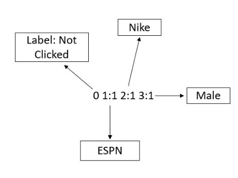
In case of a categorical field, the feature is uniquely encoded and a value of 1 is assigned to it. In the above figure ESPN is represented by code 1, Nike is represented by code 2 and so on. Each line contains an equivalent training example and is ended by a ‘\n’ or a new line character.

For classification(binary/multiclass), <label> is an integer indicating the class label.
For regression, <label> is the target value which can be any real number.
Labels in the test file are only used to calculate accuracy or errors. If they are unknown, you can just fill the first column with any number.

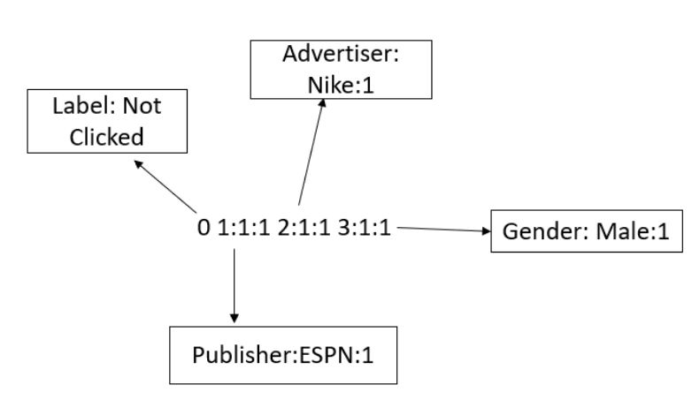
Similarly for FFMs, the data needs to be transformed to a libffm format. Here, we also need to encode the field since ffm requires the information of field for learning. The format for the same is:

<label> <field1>:<feature1>:<value1> <field2>:<feature2>:<value2> …..

Important note on numerical features

Numerical features either need to be discretized (transformed to categorical features by breaking the entire range of a particular numerical feature into smaller ranges and label encoding each range separately) and then converted to libffm format as described above.

Another possibility is to add a dummy field which is the same as feature value will be numeric feature for that particular row (For example a feature with value 45.3 can be transformed to 1:1:45.3). However, the dummy fields may not be informative because they are merely duplicates of features.

xLearn

Recently launched xLearn library provides a fast solution to implementing FM and FFM models on a variety of datasets. It is much faster than libfm and libffm libraries and provide a better functionality for model testing and tuning.

Here, we will illustrate with an example of FFM for a tiny sample(1%) of CTR dataset from Criteo’s click prediction challenge.

First, we need to convert the dataset to libffm format which is necessary for xLearn to fit the model. Following function does the job of converting dataset in standard dataframe format to libffm format.

df = Dataframe to be converted to ffm format

Type = Train/Test/Val

Numerics = list of all numeric fields

Categories = list of all categorical fields

Features = list of all features except the Label and Id

# Based on Kaggle kernel by Scirpus
def convert_to_ffm(df,type,numerics,categories,features):
    currentcode = len(numerics)
    catdict = {}
    catcodes = {}
    # Flagging categorical and numerical fields
    for x in numerics:
         catdict[x] = 0
    for x in categories:
         catdict[x] = 1
    
    nrows = df.shape[0]
    ncolumns = len(features)
    with open(str(type) + "_ffm.txt", "w") as text_file:

    # Looping over rows to convert each row to libffm format
    for n, r in enumerate(range(nrows)):
         datastring = ""
         datarow = df.iloc[r].to_dict()
         datastring += str(int(datarow['Label']))
         # For numerical fields, we are creating a dummy field here
         for i, x in enumerate(catdict.keys()):
             if(catdict[x]==0):
                 datastring = datastring + " "+str(i)+":"+ str(i)+":"+ str(datarow[x])
             else:
         # For a new field appearing in a training example
                 if(x not in catcodes):
                     catcodes[x] = {}
                     currentcode +=1
                     catcodes[x][datarow[x]] = currentcode #encoding the feature
         # For already encoded fields
                 elif(datarow[x] not in catcodes[x]):
                     currentcode +=1
                     catcodes[x][datarow[x]] = currentcode #encoding the feature
                 code = catcodes[x][datarow[x]]
                 datastring = datastring + " "+str(i)+":"+ str(int(code))+":1"

         datastring += '\n'
         text_file.write(datastring)

xLearn can handle csv as well as libsvm format for implementation of FMs while we necessarily need to convert it to libffm format for using FFM. You can download the processed dataset from here.

Once we have the dataset in libffm format, we could train the model using the xLearn library.

Similar to any other ML algorithm, the dataset is divided into a training set and a validation set. xLearn automatically performs early stopping using the validation/test logloss and we can also declare another metric and monitor on the validation set for each iteration of the stochastic gradient descent.

The following python script could be used for training and tuning hyperparameters of FFM model using xlearn on a dataset in ffm format.

import xlearn as xl

ffm_model = xl.create_ffm()
ffm_model.setTrain("criteo.tr.r100.gbdt0.ffm")
ffm_model.setValidate("criteo.va.r100.gbdt0.ffm")

param = {'task':'binary', # ‘binary’ for classification, ‘reg’ for Regression
         'k':2,           # Size of latent factor
         'lr':0.1,        # Learning rate for GD
         'lambda':0.0002, # L2 Regularization Parameter
         'Metric':'auc',  # Metric for monitoring validation set performance
         'epoch':25       # Maximum number of Epochs
        }

ffm_model.fit(param, "model.out")

The library also allows us to use cross-validation using the cv() function:

ffm_model.cv(param)

Predictions can be done on the test set with the following code snippet:

# Convert output to 0/1
ffm_model.setTest("criteo.va.r100.gbdt0.ffm")
ffm_model.setSigmoid()
ffm_model.predict("model.out", "output.txt")

End Notes

In this article we have demonstrated the usage of factorization for normal classification/Regression problems. Please let us know how this algorithm performed for your problem. Detailed documentation for xlearn is given at this link and has regular support by its contributors.