LM优化算法的Matlab实现

LM算法即Levenberg-Marquardt算法。这个优化算法的具体理论讲解以及推导在此不叙述，网上能找到好多好多的这方面的讲解，在这里推荐去wiki 上或看 K. Madsen等人的《Methods for non-linear least squares problems》文章，好吧在此附上原文链接：http://www2.imm.dtu.dk/pubdb/views/edoc_download.php/3215/pdf/imm3215.pdf

本文主要是想通过Matlab程序结合一个示例来实现一下LM算法，在此有一篇blog写的很不错，使用Matlab实现了LM算法，网址：http://blog.sina.com.cn/s/blog_4a8e595e01014tvb.html 这篇blog是转载的，本着尊重原作者的想法，本想根据这篇blog给的原作者的网址：http://www.shenlejun.cn/my/article/show.asp?id=17&page=2

却打不开，所以只好把网址贴上一并贴上，有知道原始出处告知一声，及时修改。

在此示例的程序数据来自上述blog，程序如下：

% 2015/05/22 by DQ
% LM算法
function LMDemo1
clc;
clear ;
close all;

Get_fx=@(x,a,b,y) ( a*exp(-b*x) -y);%误差函数
Get_Jx=@(x,a,b) ([ exp(-b*x),-a*exp(-b*x).*x ]);%雅可比矩阵
Get_A=@(x,a,b) ( transpose(Get_Jx(x,a,b))*Get_Jx(x,a,b) );
Get_g=@(x,a,b,y) ( transpose(Get_Jx(x,a,b))*Get_fx(x,a,b,y) );

Get_Fx=@(x,a,b,y) ( 0.5*transpose(Get_fx(x,a,b,y))*Get_fx(x,a,b,y) );%目标函数 0.5是为了方便处理系数
Get_L=@(x,a,b,y,h) ( Get_Fx(x,a,b,y)+h'*transpose(Get_Jx(x,a,b))*Get_fx(x,a,b,y)+...
    0.5*h'*Get_A(x,a,b)*h );%近似模型函数

% 拟合用数据。参见《数学试验》，p190，例2
X=[0.25 0.5 1 1.5 2 3 4 6 8]';
Y=[19.21 18.15 15.36 14.10 12.89 9.32 7.45 5.24 3.01]';

v=2;
tao=1e-10;
e1=1e-12;
e2=1e-12;
k=0;
k_max=1000;

a0=10;b0=0.5;
t=[a0;b0];
Ndim=2;
A=Get_A(X,a0,b0);
g=Get_g(X,a0,b0,Y);

found=(norm(g)<=e1);
mou=tao*max(diag(A));
while (~found &&(k<k_max))%
    k=k+1;
    h_lm=-inv(A+mou*eye(Ndim))*g;
    if (norm(h_lm)<=e2*(norm(t)+e2))
        found=true;
    else
        t_new=t+h_lm;
        Fx=Get_Fx(X,t(1),t(2),Y);
        Fx_h=Get_Fx(X,t_new(1),t_new(2),Y) ;
        L_0=Get_L(X,t(1),t(2),Y,zeros(Ndim,1));
        L_h=Get_L(X,t(1),t(2), Y,h_lm);
        rho=(Fx-Fx_h)./(L_0-L_h);
        if rho>0
            t=t_new;
            A=Get_A(X,t(1),t(2));
            g=Get_g(X,t(1),t(2),Y);
            found=(norm(g)<=e1);
            mou=mou*max([0.3333,1-(2*rho-1).^3]);
            v=2;
        else
            mou=mou*v;
            v=2*v;
        end
    end
end
k
PlotFitLine(X,Y,t);
end


function PlotFitLine(X,Y,t)
FitY=@(x,a,b) ( a*exp(-b*x) );
Y_hat=FitY(X,t(1),t(2));
figure;
plot(X,Y);
hold on;
plot(X,Y_hat,'g -*');
legend('原始数据','拟合数据');
title('LM最小二乘优化拟合');
end

运行上述程序后得到的拟合函数和原始数据的图像显示如下：

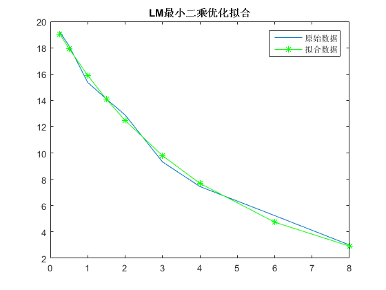
得到的最佳参数t=[20.2413 ,0.2420]；本文实现的过程和blog大同小异但收敛速度比较快，在和上述blog初始参数一致的前提下，30次以内就达到最优状态了。

LM优化算法的Matlab实现

猜你喜欢