陀螺仪随机误差的Allan方差分析

https://blog.csdn.net/u012325601/article/details/60882949

陀螺仪随机误差的Allan方差分析

GitHub仓库：https://github.com/XinLiGitHub/GyroAllan

PS：博文不再更新，后续更新会在GitHub仓库进行。

1，前言

陀螺仪的随机误差主要包括：量化噪声、角度随机游走、零偏不稳定性、角速率随机游走、速率斜坡和正弦分量。对于这些随机误差，利用常规的分析方法，例如计算样本均值和方差，并不能揭示出潜在的误差源。另一方面，在实际工作中通过对自相关函数和功率谱密度函数加以分析将随机误差分离出来是很困难的。Allan方差法是20世纪60年代由美国国家标准局的David Allan提出的，它是一种基于时域的分析方法。Allan方差法的主要特点是能非常容易地对各种误差源及其对整个噪声统计特性的贡献进行细致的表征和辨识，而且具有便于计算、易于分离等优点。

2，MATLAB程序

allan.m文件

function [T,sigma] = allan(omega,fs,pts)
[N,M] = size(omega); % figure out how big the output data set is
n = 2.^(0:floor(log2(N/2)))'; % determine largest bin size
maxN = n(end);
endLogInc = log10(maxN);
m = unique(ceil(logspace(0,endLogInc,pts)))'; % create log spaced vector average factor
t0 = 1/fs; % t0 = sample interval
T = m*t0; % T = length of time for each cluster
theta = cumsum(omega)/fs; % integration of samples over time to obtain output angle θ
sigma2 = zeros(length(T),M); % array of dimensions (cluster periods) X (#variables)
for i=1:length(m) % loop over the various cluster sizes
for k=1:N-2*m(i) % implements the summation in the AV equation
sigma2(i,:) = sigma2(i,:) + (theta(k+2*m(i),:) - 2*theta(k+m(i),:) + theta(k,:)).^2;
end
end
sigma2 = sigma2./repmat((2*T.^2.*(N-2*m)),1,M);
sigma = sqrt(sigma2);

nihe.m文件

function C=nihe(tau,sig,M)
X=tau';Y=sig';
B=zeros(1,2*M+1);
F=zeros(length(X),2*M+1);
for i=1:2*M+1
kk=i-M-1;
F(:,i)=X.^kk;
end
A=F'*F;
B=F'*Y;
C=A\B;

gyro_data.m文件

clc;
clear;
data = dlmread('data.dat'); %从文本中读取数据，单位：deg/s，速率：100Hz
data = data(720000:2520000, 3:5)*3600; %截取保温两个小时后的，五个小时的数据，把 deg/s 转为 deg/h
[A, B] = allan(data, 100, 100); %求Allan标准差，用100个点来描述
loglog(A, B, 'o'); %画双对数坐标图
xlabel('time:sec'); %添加x轴标签
ylabel('Sigma:deg/h'); %添加y轴标签
legend('X axis','Y axis','Z axis'); %添加标注
grid on; %添加网格线
hold on; %使图像不被覆盖
C(1, :) = nihe(A', (B(:,1)').^2, 2)'; %拟合
C(2, :) = nihe(A', (B(:,2)').^2, 2)';
C(3, :) = nihe(A', (B(:,3)').^2, 2)';
Q = sqrt(abs(C(:, 1) / 3)); %量化噪声，单位：deg/h
N = sqrt(abs(C(:, 2) / 1)) / 60; %角度随机游走，单位：deg/h^0.5
Bs = sqrt(abs(C(:, 3))) / 0.6643; %零偏不稳定性，单位：deg/h
K = sqrt(abs(C(:, 4) * 3)) * 60; %角速率游走，单位：deg/h/h^0.5
R = sqrt(abs(C(:, 5) * 2)) * 3600; %速率斜坡，单位：deg/h/h
fprintf('量化噪声 X轴：%f Y轴：%f Z轴：%f 单位：deg/h\n', Q(1), Q(2), Q(3));
fprintf('角度随机游走 X轴：%f Y轴：%f Z轴：%f 单位：deg/h^0.5\n', N(1), N(2), N(3));
fprintf('零偏不稳定性 X轴：%f Y轴：%f Z轴：%f 单位：deg/h\n', Bs(1), Bs(2), Bs(3));
fprintf('角速率游走 X轴：%f Y轴：%f Z轴：%f 单位：deg/h/h^0.5\n', K(1), K(2), K(3));
fprintf('速率斜坡 X轴：%f Y轴：%f Z轴：%f 单位：deg/h/h\n', R(1), R(2), R(3));
D(:, 1) = sqrt(C(1,1)*A.^(-2) + C(1,2)*A.^(-1) + C(1,3)*A.^(0) + C(1,4)*A.^(1) + C(1,5)*A.^(2)); %生成拟合函数
D(:, 2) = sqrt(C(2,1)*A.^(-2) + C(2,2)*A.^(-1) + C(2,3)*A.^(0) + C(2,4)*A.^(1) + C(2,5)*A.^(2));
D(:, 3) = sqrt(C(3,1)*A.^(-2) + C(3,2)*A.^(-1) + C(3,3)*A.^(0) + C(3,4)*A.^(1) + C(3,5)*A.^(2));
loglog(A, D); %画双对数坐标图

3，运行结果

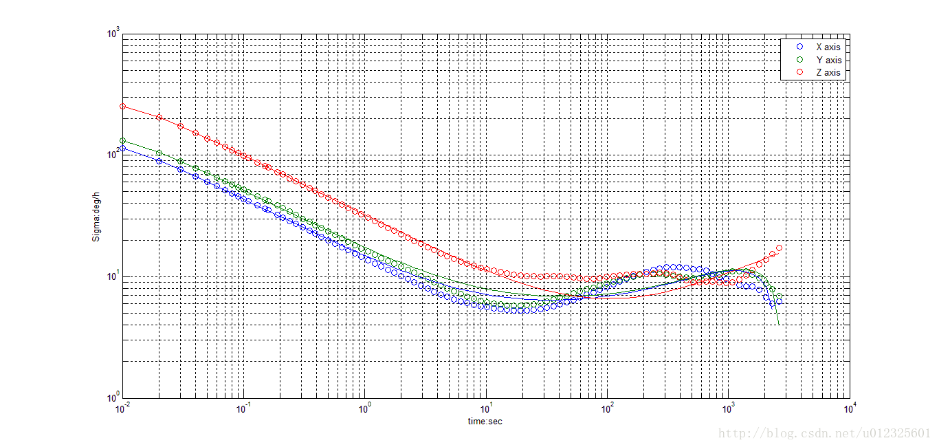
         量化噪声          X轴：0.458971 Y轴：0.564662 Z轴：1.118367 单位：deg/h
         角度随机游走 X轴：0.231291 Y轴：0.273737 Z轴：0.532305 单位：deg/h^0.5
         零偏不稳定性 X轴：8.264598 Y轴：8.849770 Z轴：7.367757 单位：deg/h
         角速率游走      X轴：42.156012 Y轴：40.870664 Z轴：32.268721 单位：deg/h/h^0.5
         速率斜坡          X轴：43.040958 Y轴：40.022454 Z轴：11.171091 单位：deg/h/h

注意：当Allan标准差的拟合多项式中的拟合系数是负值时，所得误差项的拟合结果随着相关时间的微小改变变化很大，拟合误差很大，可信度差。

陀螺仪随机误差的Allan方差分析

猜你喜欢