特征选择的探索

1. 背景知识

数据和特征决定了机器学习的上限，而模型和算法只是逼近这个上限而已。

这句话可以说是机器学习中的至理名言，出处现在已不可考。但是它时时刻刻提醒着机器学习者们数据和特征的重要性，一个好的算法可以将预测结果变好一点，但是干净的数据和合理的特征可能让你的结果有一个显著性提升。现如今越来越多的人明白了许多机器学习失败的原因，并不是因为算法的好坏（个人感觉算法没有好坏之分），而在于数据的处理和特征的选取，这篇博客，我来总结一下关于特征的选取部分，即大家耳熟能详的 特征选择 问题。

机器学习首先需要对数据进行训练，而每一个训练数据（或样本，或实例）都可看做一行特征集合组成的向量。如一个拥有 n 个特征和 1 个类标签的数据 $x$ 可以表示为，

$x = (x_{1}, x_{2}, x_{3}, ... , x_{n}, y)$

虽然直觉上来讲，维度越多（$n$ 越大），数据 $x$ 能够表示的信息就越多，模型训练的就越好。但是事实上并不是这样，当数据的维度扩张到很大时，会出现另一个问题，即 维度灾难（the curse of dimensionality），维基百科关于维度灾难的解释如下，

The curse of dimensionality refers to various phenomena that arise when analyzing and organizing data in high-dimensional spaces (often with hundreds or thousands of dimensions) that do not occur in low-dimensional settings such as the three-dimensional physical space of everyday experience 1

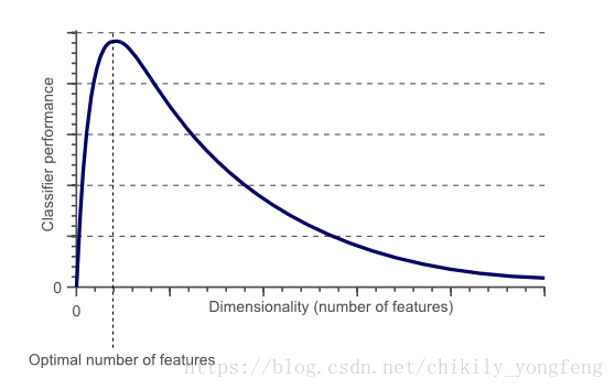
维度灾难特指由于处理高维数据空间而引发的各种问题，这里的“高维数据”一般指成百上千维的数据，而不是三维，四维这样的“低维数据”。经研究表明 2 当训练数据量固定时，分类器（或回归器）的性能随着特征维度的增加而 先上升后下降，这个现象称之为 Hughes phenomenon，或者 peaking phenomena。原因在于 大量的无关特征，冗余特征会干扰模型的训练。请参见下图。

当然，学术界还有一种观点认为 3 训练集中至少需要 5 个样本才能表示好 1 个特征。换句话说，就是 1 个特征至少对应 5 个样本，如果你的训练集中有 $n$ 个特征，那么你至少需要 $5n$ 个样本才能训练出较好的模型。

2. 特征选择

In machine learning and statistics, feature selection, also known as variable selection, attribute selection or variable subset selection, is the process of selecting a subset of relevant features (variables, predictors) for use in model construction.4

特征选择（feature selection），又称为变量选择，属性选择，或者变量子集选择。它指的是 从原始特征集中选取最优特征子集 的过程。筛选后得到的最优特征子集训练出来的模型具有更强的预测能力。特征选择的主要解决 维度灾难 问题。

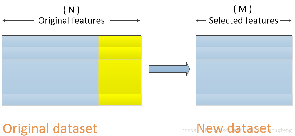
特征选择的目的是选取最优特征子集，因此对于一个数据集来讲，特征选择是在横向上（特征）做选择，竖向上（样本）保持不变，如下图所示，展现了一个拥有 N 个特征的原始数据集（Original dataset），进行特征选择之后的结果，即变成了一个拥有 M 个特征的新数据集（New dataset）。

现阶段特征选择的方法主要有 3 种，分别是 Filter 方法，Wrapper 方法，和 Embedded 方法，2.1，2.2，2.3 小节分别从原理和实现上介绍这 3 种方法。

2.1 Filter 过滤

Filter 方法针对于每个特征进行单独考量。它会对 每个特征计算得到一个评分，通过设定阈值来过滤掉那些评分低于阈值的属性。针对于分类问题，可以采用卡方检验（$\chi ^{2}$）等；对于 回归问题，可以采用皮尔森相关系数（Pearsons’ Correlation Coefficient），最大信息系数（Maximal Information Coefficient）等。

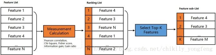
下图介绍了 Filter 方法大致过程。首先对 Feature List 中的 $n$ 个特征（Feature 1 ~ Feature N）进行评分，将其排序得到顺序特征列表 Ranking List。然后选取排名前 $k$ 个特征，或者选取大于阈值的特征。

下面用 python 来实现来过滤特征，我们需要引入 feature_selection 5 和 pandas 包。

STEP 1：从 csv 文件用 read_csv() 函数中读取数据（DataFrame 形式），并得到自变量 X 和因变量 Y。

import pandas as pd

def read_from_csv(path=codec.csv""):
    """
    read features and class from csv file
    """
    pddata = pd.read_csv(path) # read from csv
    features = pddata.columns[:-1] # define the feature
    flag = pddata.columns[-1] # define the class label

    X = [] # features list
    Y = [] # class list
    for i in range(len(pddata)):
        X.append(pddata.iloc[i][features].tolist())
        Y.append(pddata.iloc[i][flag])
    return [X, Y]

STEP 2：使用不同的系数来计算每个特征的评分，再根据阈值来获得最优特征子集 new_X，或者最优特征序号 new_X_index。

• 卡方检验（针对分类问题），这里的 chi2 也可以替换为 f_classif, mutual_info_classif 等。

from sklearn.feature_selection import SelectKBest
from sklearn.feature_selection import chi2

def select_by_chi2(X, Y, k=50):
    """
    filter the features using ChiSquared
    """
    sel = SelectKBest(chi2, k)
    # sel = SelectPercentile(chi, 0.8)
    new_X = sel.fit_transform(X, Y)
    return new_X

• 皮尔森系数（针对回归问题）

from scipy import stats

def select_by_pearson(X, Y, threashold=0.3):
    """
    filter the features using pearson's correlation coefficient
    """
    new_X_index = []
    for i in range(len(X[0])): # for each feature
        feature_i = [x[i] for x in X]
        corr = stats.pearsonr(feature_i, Y)[0] # correlation with Y 
        if corr > threshold:
            new_X_index.append(i)
    return new_X_index

• 最大信息系数（）

from minepy import MINE

def select_by_mic(X, Y, threshold):
    """
    filter the features using MIC coefficient
    """
    new_X_index = []
    for i in range(len(X[0])): # for each feature
        feature_i = [x[i] for x in X]
        m = MINE()
        m.compute_score(feature_i, Y) # mic with Y 
        mic = m.mic()
        if mic > threshold:
            new_X_index.append(i)
    return new_X_index

注：在特征选择方法里，其实也包含一种 移除低方差 的特征选择方法。它的含义是去除掉那些方差小于某一阈值的特征，因为特征的方差越小就越稳定，那么对于预测结果的辨识度也会变小。实现如下使用 VarianceThreshold() 函数。

• 低方差移除法（针对方差较小的特征）

from sklearn.feature_selection import VarianceThreshold

def select_by_variance(X, threshold=0.8):
    """
    filter the features who has lower variance
    """
    sel = VarianceThreshold(threshold*(1-threshold))
    # remove the features whose 80% values are the same
    new_X = sel.fit_transform(X)
    return new_X

2.2 Wrapper 包裹

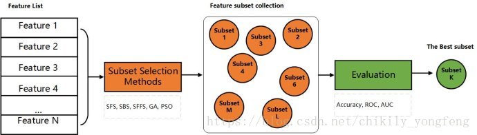
Wrapper 方法针对于整体特征集进行考量。它会进行 多轮模型训练，每一轮又通过目标函数来淘汰一批特征，或者增加一批特征。

• 递归特征移除法（Recursive feature elimination）

分批次移除特征。每轮用相同模型（如决策树 j48）对训练集进行建模，模型会对每个特征计算其权重参数 coef_，每一轮去掉 step 个权重参数最低的特征。如此反复，直到最终得到 k 个最优特征子集。

from sklearn.tree import DecisionTreeClassifier
from sklearn.feature_selection import RFE

def select_by_rfe(X, Y, k=50, step=2):
    """
    filter the features using RFE
    """
    j48 = DecisionTreeClassifier()
    rfe = RFE(estimator=j48, n_features_to_select=k, step=step)
    new_x = rfe.fit_transform(X, Y)
    # results = rfe.ranking_ # ranking of each feature
    return new_X

2.1 Embedded 内嵌

Embedded 方法其实并不是一种特征选择方法，只是借助某些分类器，回归器内部对特征的评分或排序来进行特征的选择。Embedded 方法相当于嵌入到了模型的内部。

我们使用 SelectFromModel() 函数来实现 Embeded 特征选择方法，首先使用决策树（j48）来来对特征进行排序，然后使用排序后高于阈值（1e-5）的特征来进行模型的建立。当然了这里的决策树可以换做任何对于特征有排名功能的分类器，像 SVM 等。

from sklearn.feature_selection import SelectFromModel
from sklearn.tree import DecisionTreeClassifier

def select_by_embedded(X, Y):
    """
    filter the features using j48 embedded
    """
    j48 = DecisionTreeClassifier()
    j48.fit(X, Y) # j48.feature_importances show the importance of features
    model = SelectFromModel(j48, prefit=True, threshold = 1e-5)
    new_X = model.transform(X)
    return new_X

Python 还实现了一种叫做 PipeLine() 的函数，可以直接将特征选择和建模联系起来，如首先使用 决策树 来进行特征选择，然后根据选择后的特征使用 SVM 分类器进行模型训练。.因此 PipeLine() 函数相当于一个小的集成分类器。

from sklearn.pipeline import Pipeline
from sklearn.feature_selection import SelectFromModel
from sklearn.svm import SVC
from sklearn.tree import DecisionTreeClassifier

def embedded_classifier(X, Y):
    """
    filter the features using Pipeline
    """
    j48 = DecisionTreeClassifier()
    svc = SVC()
    clf = Pipeline([
      ('feature_selection', SelectFromModel(j48)), # j48 to select feature
      ('classification', svc) # svm to train the model
    ])
    clf.fit(X, Y)
    return clf

基本的特征选择方法 Wrapper，Filter，和 Embedded 方法介绍完了，但是这些方法没有好坏之分，正如分类器也没有好坏之分一样，关键是能找到一个对的数据（需要确认眼神:）。

---

1. wikipedia. Curse of dimensionality. https://en.wikipedia.org/wiki/Curse_of_dimensionality ↩
2. Trunk, G. V. (July 1979). “A Problem of Dimensionality: A Simple Example“. IEEE Transactions on Pattern Analysis and Machine Intelligence. PAMI-1 (3): 306–307. doi:10.1109/TPAMI.1979.4766926. ↩
3. Koutroumbas, Sergios Theodoridis, Konstantinos (2008). “Pattern Recognition“. Burlington. Retrieved 8 January 2018. ↩
4. Wikipedia. Feature Selection. https://en.wikipedia.org/wiki/Feature_selection ↩
5. Scikit-learn. Feature Selection. http://scikit-learn.org/stable/modules/feature_selection.html ↩