R语言学习记录：因子分析的R实现

时间： 2018-08-09(学习时间)、2018-08-12(记录时间)
教程：知乎：Learn R | 数据降维之主成分分析（上）、Learn R | 数据降维之因子分析（下） 作者：Jason
数据来源：《应用多元统计分析》 王学民 编著 P261-P262 习题8.5、8.6

---

因子分析

1.因子分析

使用psych包对数据进行因子分析。
其中，fa函数进行主成分分析，fa.parallel函数生成碎石图。

fa(r, nfactors=, n.obs=, rotate=, scores=, fm=) r:相关系数矩阵或原始数据矩阵，
nfactors:设定主提取的因子数（默认为1） n.obs:观测数（输入相关系数矩阵时需要填写）
rotate:设定旋转的方法（默认互变异数最小法） scores:设定是否需要计算因子得分（默认不需要）
fm:设定因子化方法（默认极小残差法）

提取公因子的方法（fm），方法包括： ml：最大似然法 pa：主轴迭代法 wls：加权最小二乘法 gls：广义加权最小二乘法
minres：最小残差法
（摘自教程）

如：

 # 导入数据
> library(openxlsx)
> data1 <- read.xlsx("E:\\Learning_R\\因子分析\\exec8.5.xlsx",rows = 1:13, cols = 1:5 )
> head(data1)
  人口 教育 佣人 服务  房价
1 5700 12.8 2500  270 25000
2 1000 10.9  600   10 10000
3 3400  8.8 1000   10  9000
4 3800 13.6 1700  140 25000
5 4000 12.8 1600  140 25000
6 8200  8.3 2600   60 12000
> data1_cor <- cor(data1)
> head(cor(data1),3)
           人口       教育      佣人      服务       房价
人口 1.00000000 0.00975059 0.9724483 0.4388708 0.02241157
教育 0.00975059 1.00000000 0.1542838 0.6914082 0.86307009
佣人 0.97244826 0.15428378 1.0000000 0.5147184 0.12192599
# 生成碎石图
> library(psych)
> fa.parallel(data1_cor, n.obs = 112, fa = "both", n.iter = 100)
Parallel analysis suggests that the number of factors =  2  and the number of components =  2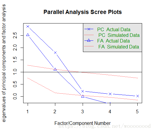 

从图中和函数给出的信息可以看出，保留两个主成分即可。

# 因子分析
> fa_model1 <- fa(data1_cor, nfactors = 2, rotate = "none", fm = "ml")
> fa_model1
Factor Analysis using method =  ml
Call: fa(r = data1_cor, nfactors = 2, rotate = "none", fm = "ml")
Standardized loadings (pattern matrix) based upon correlation matrix
       ML2  ML1   h2    u2 com
人口 -0.03 1.00 1.00 0.005 1.0
教育  0.90 0.04 0.81 0.193 1.0
佣人  0.09 0.98 0.96 0.036 1.0
服务  0.78 0.46 0.81 0.185 1.6
房价  0.96 0.05 0.93 0.074 1.0

                       ML2  ML1
SS loadings           2.34 2.16
Proportion Var        0.47 0.43
Cumulative Var        0.47 0.90
Proportion Explained  0.52 0.48
Cumulative Proportion 0.52 1.00

Mean item complexity =  1.1
Test of the hypothesis that 2 factors are sufficient.

The degrees of freedom for the null model are  10  and the objective function was  6.38
The degrees of freedom for the model are 1  and the objective function was  0.31 

The root mean square of the residuals (RMSR) is  0.01 
The df corrected root mean square of the residuals is  0.05 

Fit based upon off diagonal values = 1
Measures of factor score adequacy             
                                                   ML2  ML1
Correlation of (regression) scores with factors   0.98 1.00
Multiple R square of scores with factors          0.95 1.00
Minimum correlation of possible factor scores     0.91 0.99

fa函数中，第一个参数是数据，第二个参数说明要保留两个主成分，第三个参数为旋转方法，为none，即不进行主成分旋转，第四个参数表示提取公因子的方法为最大似然法。
输出结果中与主成分输出结果基本一致，可以看出该数据选取两个主成分解释了原始5个变量的90%的方差。

# 因子旋转：正交旋转法
> fa_model2 <- fa(data1_cor, nfactors = 2, rotate = "varimax", fm = "ml")
> fa_model2
Factor Analysis using method =  ml
Call: fa(r = data1_cor, nfactors = 2, rotate = "varimax", fm = "ml")
Standardized loadings (pattern matrix) based upon correlation matrix
      ML2  ML1   h2    u2 com
人口 0.02 1.00 1.00 0.005 1.0
教育 0.90 0.00 0.81 0.193 1.0
佣人 0.14 0.97 0.96 0.036 1.0
服务 0.80 0.42 0.81 0.185 1.5
房价 0.96 0.00 0.93 0.074 1.0

                       ML2  ML1
SS loadings           2.39 2.12
Proportion Var        0.48 0.42
Cumulative Var        0.48 0.90
Proportion Explained  0.53 0.47
Cumulative Proportion 0.53 1.00

Mean item complexity =  1.1
Test of the hypothesis that 2 factors are sufficient.

The degrees of freedom for the null model are  10  and the objective function was  6.38
The degrees of freedom for the model are 1  and the objective function was  0.31 

The root mean square of the residuals (RMSR) is  0.01 
The df corrected root mean square of the residuals is  0.05 

Fit based upon off diagonal values = 1
Measures of factor score adequacy             
                                                   ML2  ML1
Correlation of (regression) scores with factors   0.98 1.00
Multiple R square of scores with factors          0.95 1.00
Minimum correlation of possible factor scores     0.91 0.99
> fa_model2$weights
            ML2          ML1
人口 -0.2023403  0.887108659
教育  0.2178564 -0.009363652
佣人  0.1241204  0.113241682
服务  0.1974628  0.001662584
房价  0.6101433 -0.025881048

rotate = varimax表示旋转方式为正交因子旋转。
由输出结果可以看出，两个因子的方差比例不变，但在各观测值上的载荷发生了改变，
data1_pca_xz$weights的内容为因子与原始变量之间之间线性回归方程的系数。

主成分分析中，主成分可以表示为原始变量的线性组合，原始变量也可以表示为因子的线性组合；而在因子分析中，原始变量是因子的线性组合，因子却不能表示为主成分的线性组合。

使用factor.plot函数对旋转结果进行可视化：

> factor.plot(fa_model2)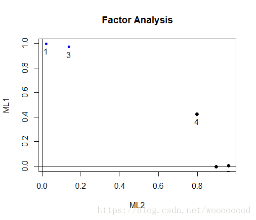

> fa.diagram(fa_model2, simple = FALSE)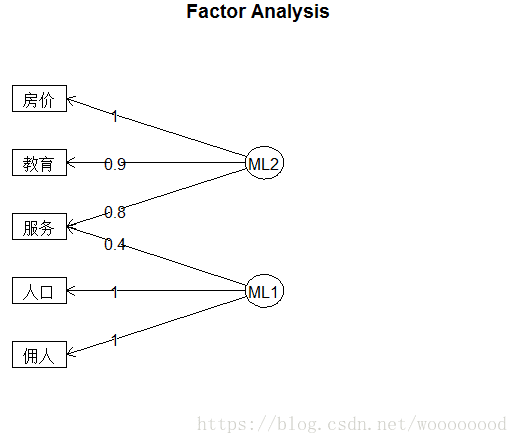

由上述结果和分析可知，该数据可以取两个因子，f1因子是与地区的房价水平、教育水平和各种服务行业的人数有主要关系的地区经济发达因子，而f2因子是与地区的总人口数和雇佣人口数有主要关系的地区人口规模因子。

2.练习

练习内容：《应用多元统计分析》 王学民 编著 P260-P261 习题8.6
数据内容：某公司老板对48名应聘者进行命面试，并给出他们在15个方面所得的分数，这15个方面分别为：申请书的形式、外貌、专业能力、讨人喜欢、自信心、精明、诚实、推销能力、经验、积极性、抱负、理解能力、潜力、交际能力和适应性。
代码及结果：

> library(openxlsx)
> data2 <- read.xlsx("E:\\Learning_R\\因子分析\\exec8.6.xlsx",rows = 1:49, cols = 1:15 )
> head(data2)
  申请 外貌 专业 讨喜 自信 精明 诚实 推销 经验 积极 抱负 理解 潜力
1    6    7    2    5    8    7    8    8    3    8    9    7    5
2    9   10    5    8   10    9    9   10    5    9    9    8    8
3    7    8    3    6    9    8    9    7    4    9    9    8    6
4    5    6    8    5    6    5    9    2    8    4    5    8    7
5    6    8    8    8    4    4    9    2    8    5    5    8    8
6    7    7    7    6    8    7   10    5    9    6    5    8    6
  交际 适应
1    7   10
2    8   10
3    8   10
4    6    5
5    7    7
6    6    6
> data2_cor <- cor(data2)
> library(psych)
> fa.parallel(data2_cor, n.obs = 112, fa = "both", n.iter = 100)
Parallel analysis suggests that the number of factors =  4  and the number of components =  3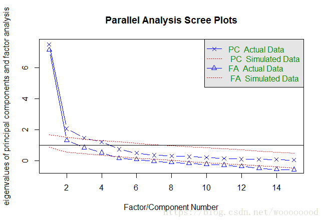 

由函数信息可知选取4个因子即可，但根据碎石图中曲线斜率来看，选取5个因子更为合适。

> fa_model4 <- fa(data2_cor, nfactors = 5, rotate = "varimax", fm = "pa")
> fa_model4
Factor Analysis using method =  pa
Call: fa(r = data2_cor, nfactors = 5, rotate = "varimax", fm = "pa")
Standardized loadings (pattern matrix) based upon correlation matrix
      PA1   PA2   PA3   PA5   PA4   h2       u2 com
申请 0.13  0.72  0.09  0.07 -0.10 0.55  0.44528 1.2
外貌 0.32  0.15  0.23  0.93  0.07 1.05 -0.05444 1.4
专业 0.06  0.13 -0.01  0.04  0.68 0.48  0.51909 1.1
讨喜 0.22  0.24  0.83  0.10 -0.06 0.82  0.18441 1.4
自信 0.90 -0.09  0.16  0.14 -0.07 0.87  0.12895 1.1
精明 0.85  0.12  0.29  0.02  0.05 0.82  0.18211 1.3
诚实 0.23 -0.22  0.75  0.14 -0.01 0.68  0.32043 1.5
推销 0.89  0.23  0.07  0.15 -0.06 0.88  0.12234 1.2
经验 0.09  0.79 -0.04 -0.01  0.21 0.68  0.32457 1.2
积极 0.77  0.37  0.19  0.01 -0.02 0.77  0.23364 1.6
抱负 0.88  0.18  0.07  0.24 -0.07 0.88  0.12430 1.3
理解 0.78  0.27  0.34  0.13  0.17 0.84  0.15532 1.8
潜力 0.72  0.34  0.43  0.11  0.27 0.92  0.08076 2.6
交际 0.44  0.39  0.56  0.00 -0.58 1.00  0.00027 3.6
适应 0.35  0.78  0.06  0.13  0.09 0.76  0.24244 1.5

                       PA1  PA2  PA3  PA5  PA4
SS loadings           5.38 2.47 2.09 1.05 0.99
Proportion Var        0.36 0.16 0.14 0.07 0.07
Cumulative Var        0.36 0.52 0.66 0.73 0.80
Proportion Explained  0.45 0.21 0.17 0.09 0.08
Cumulative Proportion 0.45 0.65 0.83 0.92 1.00

Mean item complexity =  1.6
Test of the hypothesis that 5 factors are sufficient.

The degrees of freedom for the null model are  105  and the objective function was  15.75
The degrees of freedom for the model are 40  and the objective function was  1.9 

The root mean square of the residuals (RMSR) is  0.02 
The df corrected root mean square of the residuals is  0.04 

Fit based upon off diagonal values = 1

为了便于解释，我们对因子进行了因子旋转，从结果可以看出，自信心、精明、推销能力、积极性、抱负、理解能力和潜力在第一个因子上载荷较大，我们可以将第一因子定义为进取能干；申请书的形式、经验和适应性在第二个因子上载荷较大，我们可以将第二因子定义为经验；讨人喜欢、诚实、潜力和交际能力在第三个因子上载荷较大，我们可以将第三因子定义为内在品质；专业能力和交际能力在第四个因子上载荷较大，我们可以将第四因子定义为外貌；外貌在在第五个因子上载荷较大，我们可以将第五因子定义为外貌。

> factor.plot(fa_model4)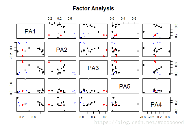

> fa.diagram(fa_model3, simple = FALSE)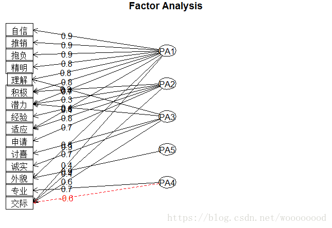

因子分析图的解释略。

> fa_model3$weights
             PA1          PA2
人口 -0.66534374  1.247355565
教育 -0.03266863  0.152682328
佣人  0.64113113 -0.253338929
服务  0.09545333  0.004111142
房价  0.87248431 -0.139003564

原始变量与因子的线性表达式略。