ensorflow 是 google 开源的机器学习工具,在2015年11月其实现正式开源,开源协议Apache 2.0。
Tensorflow特点
-
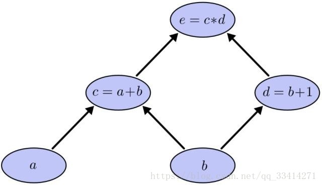
使用图 (graph) 来表示计算任务.
如图计算两个数之和的乘积(a+b)*(b+1) -
在被称之为 会话 (Session) 的上下文 (context) 中执行图.
-
使用 tensor 表示数据.
-
通过 变量 (Variable) 维护状态.
-
使用 feed 和 fetch 可以为任意的操作(arbitrary operation) 赋值或者从其中获取数据.
MNIST上基本分类操作
导入数据
from tensorflow.examples.tutorials.mnist import input_data
mnist = input_data.read_data_sets("MNIST_data/", one_hot=True)
import tensorflow as tf- 1
- 2
- 3
创建session
Tensorflow依赖于一个高效的C++后端来进行计算。
与后端的这个连接叫做session。
一般而言,使用TensorFlow程序的流程是先创建一个图,然后在session中启动它。
sess = tf.InteractiveSession()- 1
构建模型
'''
我们通过为输入图像和目标输出类别创建节点,来开始构建计算图。

784是一张展平的MNIST图片的维度
'''
x = tf.placeholder("float", shape=[None, 784])
y_ = tf.placeholder("float", shape=[None, 10])
#为模型定义权重W和偏置b
W = tf.Variable(tf.zeros([784,10]))
b = tf.Variable(tf.zeros([10]))
#变量需要通过seesion初始化后,才能在session中使用。
sess.run(tf.initialize_all_variables())

'''
类别预测与损失函数
'''
y = tf.nn.softmax(tf.matmul(x,W) + b)
cross_entropy = -tf.reduce_sum(y_*tf.log(y))
- 1
- 2
- 3
- 4
- 5
- 6
- 7
- 8
- 9
- 10
- 11
- 12
- 13
- 14
- 15
- 16
- 17
- 18
- 19
训练
train_step = tf.train.GradientDescentOptimizer(0.01).minimize(cross_entropy)
#每一步迭代,我们都会加载50个训练样本,然后执行一次train_step,并通过feed_dict将x 和 y_张量占位符用训练训练数据替代。
for i in range(1000):
  batch = mnist.train.next_batch(50)
train_step.run(feed_dict={x: batch[0], y_: batch[1]})- 1
- 2
- 3
- 4
- 5
评估
correct_prediction = tf.equal(tf.argmax(y,1), tf.argmax(y_,1))# tf.equal 来检测我们的预测是否真实标签匹配(索引位置一样表示匹配)。
accuracy = tf.reduce_mean(tf.cast(correct_prediction, "float"))#将布尔值转换为浮点数来代表对、错,然后取平均值。例如:[True, False, True, True]变为[1,0,1,1],计算出平均值为0.75。
#计算出在测试数据上的准确率,大概是91%。
print (accuracy.eval(feed_dict={x: mnist.test.images, y_: mnist.test.labels}))- 1
- 2
- 3
- 4
计算出在测试数据上的准确率,大概是91%。
MNIST上使用CNN结果
构建一个多层卷积网络
权重初始化
def weight_variable(shape):
  initial = tf.truncated_normal(shape, stddev=0.1)
  return tf.Variable(initial)

def bias_variable(shape):
  initial = tf.constant(0.1, shape=shape)
return tf.Variable(initial)- 1
- 2
- 3
- 4
- 5
- 6
- 7
卷积和池化
def conv2d(x, W):
  return tf.nn.conv2d(x, W, strides=[1, 1, 1, 1], padding='SAME')

def max_pool_2x2(x):
  return tf.nn.max_pool(x, ksize=[1, 2, 2, 1],
strides=[1, 2, 2, 1], padding='SAME')- 1
- 2
- 3
- 4
- 5
- 6
第一层卷积
一个卷积接一个max pooling完成。卷积在每个5x5的patch中算出32个特征。
卷积的权重张量形状是[5, 5, 1, 32],
前两个维度是patch的大小,接着是输入的通道数目,最后是输出的通道数目。
而对于每一个输出通道都有一个对应的偏置量。
W_conv1=weight_variable([5,5,1,32])
b_conv1=bias_variable([32])

#x变成一个4d向量,其第2、第3维对应图片的宽、高,
#最后一维代表图片的颜色通道数(因为是灰度图所以这里的通道数为1,如果是rgb彩色图,则为3
x_image=tf.reshape(x,[-1,28,28,1])

#把x_image和权值向量进行卷积,加上偏置项,然后应用ReLU激活函数,最后进行max pooling。
h_conv1=tf.nn.relu(conv2d(x_image,W_conv1)+b_conv1)
h_pool1=max_pool_2x2(h_conv1)- 1
- 2
- 3
- 4
- 5
- 6
- 7
- 8
- 9
- 10
第二层卷积
为了构建一个更深的网络,我们会把几个类似的层堆叠起来。第二层中,每个5x5的patch会得到64个特征。
W_conv2=weight_variable([5,5,32,64])
b_conv2=bias_variable([64])

h_conv2=tf.nn.relu(conv2d(h_pool1,W_conv2)+b_conv2)
h_pool2=max_pool_2x2(h_conv2)- 1
- 2
- 3
- 4
- 5
密集连接层
现在,图片尺寸减小到7x7,我们加入一个有1024个神经元的全连接层,用于处理整个图片。
我们把池化层输出的张量reshape成一些向量,乘上权重矩阵,加上偏置,然后对其使用ReLU。
W_fc1=weight_variable([7*7*64,1024])
b_fc1=bias_variable([1024])

h_pool2_flat=tf.reshape(h_pool2,[-1,7*7*64])
h_fc1=tf.nn.relu(tf.matmul(h_pool2_flat,W_fc1)+b_fc1)- 1
- 2
- 3
- 4
- 5
为了减少过拟合,我们在输出层之前加入dropout。
我们用一个placeholder来代表一个神经元的输出在dropout中保持不变的概率。
这样我们可以在训练过程中启用dropout,在测试过程中关闭dropout。
keep_prob=tf.placeholder('float')
h_fc1_drop=tf.nn.dropout(h_fc1,keep_prob)- 1
- 2
输出层
W_fc2=weight_variable([1024,10])
b_fc2=bias_variable([10])

y_conv=tf.nn.softmax(tf.matmul(h_fc1_drop,W_fc2)+b_fc2)- 1
- 2
- 3
- 4
训练和评估模型
在feed_dict中加入额外的参数keep_prob来控制dropout比例。然后每100次迭代输出一次日志。
会用更加复杂的ADAM优化器来做梯度最速下降
cross_entropy = -tf.reduce_sum(y_*tf.log(y_conv))
train_step = tf.train.AdamOptimizer(1e-4).minimize(cross_entropy)
correct_prediction = tf.equal(tf.argmax(y_conv,1), tf.argmax(y_,1))
accuracy = tf.reduce_mean(tf.cast(correct_prediction, "float"))
sess.run(tf.initialize_all_variables())
for i in range(20000):
  batch = mnist.train.next_batch(50)
  if i%100 == 0:
    train_accuracy = accuracy.eval(feed_dict={
        x:batch[0], y_: batch[1], keep_prob: 1.0})
    print ("step %d, training accuracy %g"%(i, train_accuracy))
  train_step.run(feed_dict={x: batch[0], y_: batch[1], keep_prob: 0.5})

print ("test accuracy %g"%accuracy.eval(feed_dict={
    x: mnist.test.images, y_: mnist.test.labels, keep_prob: 1.0}))