《deep learning for cv with python start bundle》第九章读书笔记

本章主要讲优化函数以及正则化

一.Vanilla gradient descent与SGD

梯度下降方法是opt【优化函数】之一

1.1Vanilla gradient descent与SGD概念

Vanilla gradient descent是原版的梯度下降，SGD对于原版进行了改进，添加了batch_size

从而使得：Vanilla gradient descent每个epoch更新一次权重，但是SGD是每个batch更新一次权重，因此每个epoch更新多次权重，因此大大加快了训练时间

引用这篇文章的内容就是：

https://stats.stackexchange.com/questions/295180/what-does-vanilla-mean

Vanilla means standard, usual, or unmodified version of something. Vanilla gradient descent means the basic gradient descent algorithm without any bells or whistles.

There are many variants on gradient descent. In usual gradient descent (also known as batch gradient descent or vanilla gradient descent), the gradient is computed as the average of the gradient of each datapoint.

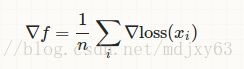
In stochastic gradient descent with a batch size of one, we might estimate the gradient as

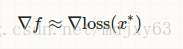
, where x∗ is randomly sampled from our entire dataset. It is a variant of normal gradient descent, so it wouldn't be vanilla gradient descent. However, since even stochastic gradient descent has many variants, you might call this "vanilla stochastic gradient descent", when comparing it to other fancier SGD alternatives, for example, SGD with momentum.

1.2：代码

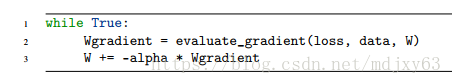
1）Vanilla gradient descent

这段是原版梯度下降的伪代码

2）SGD

伪代码实现

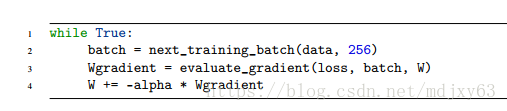
和上面标准的梯度下降算法的唯一不同点是：引入了next_training_batch,将整个数据集进行了拆分成多个batch

3)融合了标准梯度下降以及SGD的python代码：

# -*- coding:utf-8 -*- 
__author__ = 'xuy'

"""
三种梯度下降的区别:梯度下降，随机梯度下降，mini batch GD
https://blog.csdn.net/u012507022/article/details/54176144
基于python实现3种梯度下降方法:
http://lib.csdn.net/article/python/64696
这段代码主要实现了GD以及SGD
"""
from sklearn.model_selection import train_test_split
from sklearn.metrics import classification_report
# A function used to create "blobs" of normally distributed data points, a handy function when testing or implementing our own models from scratch.
#make_blobs的使用教程：https://blog.csdn.net/ichuzhen/article/details/51768934
from sklearn.datasets import make_blobs

import numpy as np
import matplotlib.pyplot as plt
import argparse



def sigmoid(x):
	""" Compute the sigmoid activation value for a given input."""
	return 1.0 / (1+np.exp(-x))


def predict(X,W):
    # Take the dot product between features and weight matrix.
    preds=sigmoid(X.dot(W))
    # Apply a step function to threshold the outputs to binary class labels.
    preds[preds<=0.5]=0
    preds[preds>0.5]=1
    return preds


#进行批处理，next_batch=当前的index+batch_size
def next_batch(X, y, batchSize):
    # Loop over dataset 'X' in mini-batches, yielding a tuple of the current batched data and labels.
    for i in np.arange(0, X.shape[0], batchSize):
        yield(X[i:i+batchSize], y[i:i+batchSize])


def main():
    ap = argparse.ArgumentParser()
    ap.add_argument("-e", "--epochs",     type=float, default=10000000,  help="# of epochs")
    ap.add_argument("-a", "--alpha",      type=float, default=0.01, help="learning rate")
    ap.add_argument("-b", "--batch_size", type=int, help="size of SGD mini-batches")
    args = vars(ap.parse_args())

    # Generate a 2-class classification problem with 1,000 data points, where each data point is a 2D feature vector.
    #此时生成的X是（1000,2），因为n_samples=1000，n_features=2
    #y是（1000，）1行1000列，需要reshape成为（1000,1）
    (X, y) = make_blobs(n_samples=1000, n_features=2, centers=2, cluster_std=1.5, random_state=1)#一共1000个点，总的特征数是2，被分为2类，方差设置为1.5，设置seed为常数【每次运行都是相同的值】
    #print('y的shape：',y.shape)#y的shape： (1000,)

    y = y.reshape((y.shape[0], 1))#变成2维,变成了（1000,1）
    # print('reshape之后y的shape：', y.shape)#reshape之后y的shape： (1000, 1)
    # Insert a column of 1's as the last entry in the feature matrix -- as the bias dimension.
    # np.c_[] -- Translates slice objects to concatenation along the second axis.
    print("x在添加1列之前的shape:",X.shape)#x在添加1列之前的shape: (1000, 2)
    X = np.c_[X, np.ones((X.shape[0]))]#在最后新添加一行全1的值，作用是当作偏执值
    print("x在添加1列之后的shape:", X.shape)#x在添加1列之后的shape: (1000, 3)

    # Partition the data into training and testing splits using 50% of the data for training and the remaining 50% for testing.
    (trainX, testX, trainY, testY) = train_test_split(X, y, test_size=0.5, random_state=42)

    # Initialize our weight matrix and list of losses.
    print("[INFO] training...")
    W = np.random.randn(X.shape[1], 1)
    print("W的shape",W.shape)#W的shape (3, 1)


    # A list that keep track of losses after each epoch for plot loss later.
    losses = []
    #mini-batch SGD的实现
    if args["batch_size"]:
        #计算每次迭代的loss
        for epoch in np.arange(0, args["epochs"]):
            # Initialize the total loss for the epoch.
            #用来保存每次batch——size的loss
            epochLoss = []
            # Loop over data in batches.
            for (batchX, batchY) in next_batch(X, y ,args["batch_size"]):#进行了一下批处理
                # Take the dot product between current batch of features and the weight matrix, then pass this value through
                #activation function
                preds = sigmoid(batchX.dot(W))#X的shape是：(1000, 3)，W的shape是（3, 1)，因此preds是（1000,1）
                error = preds - batchY#计算误差，shape是（1000,1）


                epochLoss.append(np.sum(error**2))#二阶loss,epochLoss是记录一次epoch当中每批batch_size的loss，np.sum(np.square(error))是一个数值

                gradient = batchX.T.dot(error)#batchX进行转置之后，shape(3,1000),error的shape是（1000,1），因此梯度的shape:(3,1)
                W += -args["alpha"] * gradient

            # Update loss history by taking the average loss across all batches.
            loss = np.average(epochLoss)#这里的loss是进行一次epochloss的平均值
            losses.append(loss)

            # Check to see if an update should be displayed.
            if epoch == 0 or (epoch + 1) % 5 == 0:#每5次进行一下输出
                print("[INFO] epoch={} , loss={:.7f}".format(int(epoch + 1), loss))
    #普通的梯度下降算法,因为没有batch_size，因此会计算整个数据集，这样耗时比较大
    else:
        # Loop over the desired number of epochs.
        for epoch in np.arange(0, args["epochs"]):
        # for epoch in np.arange(0, 200):
            # Take the dot product between features 'X' and the weight matrix 'W', then pass this value through our sigmoid
            #activation function, thereby giving predictions on the dataset.
            preds = sigmoid(trainX.dot(W))

            # Computing the 'error' which is the difference between predictions and the ground-true label values.
            error = preds - trainY#error的shape=（1000,1）
            # MSE(mean square error) of each data point.
            loss = np.sum(error**2)#loss是一个数值
            losses.append( loss)


            # The gradient descent update is the dot product between features and the error of the predictions.
            gradient = trainX.T.dot(error)#trainX.T.shape=(3,1000),error.shape=(1000,1),最终gradient的shape是（3,1）
            # In the update stage, all we need to do is "nudge" the weight matrix in the negative direction of the gradient(
            #hence the term 'gradient descent' by taking a small step towards a set of 'more optimal' parameters.
            W += -args["alpha"] * gradient

            # print("losses的shape是",losses.shape)

            # Check to see if an update should be displayed.
            if epoch == 0 or (epoch + 1) % 5 == 0:
                print("[INFO] epoch={} , loss={:.7f}".format(int(epoch+1), loss))

    # Evaluate model，对于结果生成报告
    print("[INFO] evaluating...")
    preds = predict(testX, W)
    print(classification_report(testY, preds))

    # Plot the testing classification data，对于test输出分类图
    plt.style.use("ggplot")
    plt.figure()
    plt.title("Data")

    colors = testY.reshape(1, testY.shape[0])[0]

    plt.scatter(testX[:, 0], testX[:, 1], marker="o", c=colors, s=30)
    plt.show()

    # Construct a figure that plots the loss over time.输出loss-time图
    plt.style.use("ggplot")
    plt.figure()
    plt.plot(np.arange(0, args["epochs"]), losses)
    plt.title("Training Loss")
    plt.xlabel("Epoch #")
    plt.ylabel("Loss")
    plt.show()


if __name__ == "__main__":
    main()

二.正则化

参考链接：https://blog.csdn.net/liujiandu101/article/details/55103831

正则化主要是利用惩罚项来限制模型过拟合

提高模型的泛化能力。主要体现在更新loss以及更新权重

2,1正则化的种类
1）数据增强

数据集合扩充

防止过拟合最有效的方法是增加训练集合，训练集合越大过拟合概率越小。数据集合扩充是一个省时有效的方法，但是在不同领域方法不太通用。 
1. 在目标识别领域常用的方法是将图片进行旋转、缩放等（图片变换的前提是通过变换不能改变图片所属类别，例如手写数字识别，类别6和9进行旋转后容易改变类目） 
2. 语音识别中对输入数据添加随机噪声 
3. NLP中常用思路是进行近义词替换 
4. 噪声注入，可以对输入添加噪声，也可以对隐藏层或者输出层添加噪声。例如对于softmax 分类问题可以通过 Label Smoothing技术添加噪声，对于类目0-1添加噪声，则对应概率变成

2）early stopping

提前停止（Early Stopping）

在模型训练过程中经常出现随着不断迭代，训练误差不断减少，但是验证误差减少后开始增长。 
提前停止（Early Stopping）的策略是：在验证误差不在提升后，提前结束训练；而不是一直等待验证误差到最小值。

1. 提前停止策略使用起来非常方便，不需要改变原有损失函数，简单而且执行效率高。
2. 但是它需要一个额外的空间来备份一份参数
3. 提前停止策略可以和其他正则化策略一起使用。
4. 提前停止策略确定训练迭代次数后，有两种策略来充分利用训练数据，一是将全量训练数据一起训练一定迭代次数；二是迭代训练流程直到训练误差小于提前停止策略的验证误差。
5. 对于二次优化目标和线性模型，提前停止策略相当于L2正则化。

3）dropout:

Dropout

Dropout是一类通用并且计算简洁的正则化方法，在2014年被提出后广泛的使用。 
简单的说，Dropout在训练过程中，随机的丢弃一部分输入，此时丢弃部分对应的参数不会更新。相当于Dropout是一个集成方法，将所有子网络结果进行合并，通过随机丢弃输入可以得到各种子网络。例如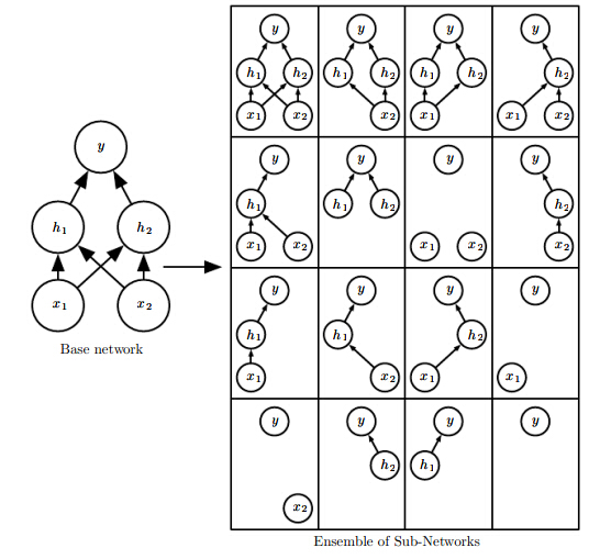 
 
例如上图，通过不同的输入屏蔽相当于学习到所有子网络结构。

因此前向传播过程变成如下形式： 
 
相当于每层输入多了一个屏蔽向量来控制该层有哪些输入会被屏蔽掉。

经验：原始输入每一个节点选择概率0.8，隐藏层选择概率为0.5

Dropout预测策略

既然Dropout过程类似于集成方法，预测时需要将所有相关模型进行求平均，对于Dropout而言，然而遍历所有屏蔽变量不是可能的事情，因此需要一些策略进行预测。 
1. 随机选择10-20个屏蔽向量就可以得到一个较好的解。 
2. 采用几何平均然后在归一化的思路。

因此只要估计出，2012年Hinton给出一种估计方法，可以只需要一遍前向传播计算最终估计值，模型参数乘上其对应输入单元被包含的概率。该方法也被称为“Weight scaling inference rule” 
3. 由于隐藏层节点drop的概率常选取0.5，因此模型权重常常除2即可；也可以在训练阶段将模型参数乘上2

dropout预测实例

假设对于多分类问题，采用softmax进行多分类，假设只有一个隐藏层，输入变量为v，输入的屏蔽变量为 d，d元素选取概率为1/2. 
则有 

d*v 代表对应元素相乘，根据几何平均，需要估计 

每一步推导基本上都是公式代入的过程，仔细一点看懂没问题。 
最后一步需要遍历所有的屏蔽向量d，然而完全遍历并且累加后可以得到2^n-1，在除以2^n，最后得到1/2. 
简单以二维举例，则d可以选择的范围包括(0,0)(0,1)(1,0)(1,1)则每一维度都累加了2次，除以4可以得到1/2

DROPOUT的优点

1. 相比于weight decay、范数约束等，该策略更有效
2. 计算复杂度低，实现简单而且可以用于其他非深度学习模型
3. 但是当训练数据较少时，效果不好
4. dropout训练过程中的随机过程不是充分也不是必要条件，可以构造不变的屏蔽参数，也能够得到足够好的解。

2.2利用多个正则项训练图片分类

主要利用SGDClassifer来进行分类，主要用到了loss function,learning rate,epoch,正则项的概念

# -*- coding:utf-8 -*- 
__author__ = 'xuy'


from sklearn.linear_model import SGDClassifier
from sklearn.preprocessing import LabelEncoder
from sklearn.model_selection import train_test_split


from pyimagesearch.preprocessing import SimplePreprocessor
from pyimagesearch.datasets import SimpleDatasetLoader
from imutils import paths

import argparse
"""
利用了animals dataset
"""
# Construct the argument parse and parse the arguments.
ap = argparse.ArgumentParser()
ap.add_argument("-d", "--dataset", required=True, help="path to input dataset")
args = vars(ap.parse_args())

# Grab the list of image paths.
print("[INFO] loading images...")
imagePaths = list(paths.list_images(args["dataset"]))

# Initialize the image preprocessor, load the dataset from disk and reshape the data matrix(flatten).
sp = SimplePreprocessor(32, 32)
sdl = SimpleDatasetLoader(preprocessors=[sp])
(data, labels) = sdl.load(imagePaths, verbose=500)
data = data.reshape((data.shape[0], -1))

# Encode the labels as integers.
le = LabelEncoder()
labels = le.fit_transform(labels)

# Partition the data into training and testing splits using 75% of the data for training and the remaining 25% for testing.
(trainX, testX, trainY, testY) = train_test_split(data, labels, test_size=0.25, random_state=5)

# Loop over dataset of regularizers
for r in (None, "l1", "l2"):#r是罚分项的种类
    # Train a SGD classifier using a softmax loss function and the specified regularization function for 10 epochs.
    print("[INFO] training model with {} 'regularization penalty term'".format(r))
    model = SGDClassifier(loss='log', penalty=r, max_iter=10, learning_rate="constant", eta0=0.01, random_state=42)#不同的random_state产生的准确率结果不同,该函数包含了loss function,epoch次数，lr,正则项
    model.fit(trainX, trainY)

    # Evaluate the classifier.
    acc = model.score(testX, testY)
    print("[INFO] '{}' regularization penalty accuracy: {:.2f}% \n".format(r, acc * 100))