tensorflow（8）tensorboard网络结构

手撕代码网络搭建完成后

1.查看网络结构（所搭建网络结构可视化）

可视化不同则代码不同，命名的地方不同：

import tensorflow as tf
from tensorflow.examples.tutorials.mnist import input_data#载入数据(可以是某盘的绝对路径)（我的数据存储在运行路径下）#可视化（暂时不关心结果，只关心结构）
#载入数据
mnist = input_data.read_data_sets('MNIST_data',one_hot = True)


 
#每个批次100张照片 每个批次的大小
batch_size = 100
 
#计算一共有多少个批次 （整除符号）
n_batch = mnist.train.num_examples // batch_size

#定义一个命名空间
with tf.name_scope('input'):
#x,y注意缩进
    #定义两个placeholder，None=100批次，重新命名
    x = tf.placeholder(tf.float32,[None,784],name='x-input')
    y = tf.placeholder(tf.float32,[None,10],name='y-input')
    
with tf.name_scope('layer'):
    #创建一个简单的神经网络（这里只是2层）
    #输入层784个神经元，输出层10个神经元
    with tf.name_scope('weights'):
        W = tf.Variable(tf.zeros([784,10]),name='W')
    with tf.name_scope('biases'):
        b = tf.Variable(tf.zeros([10]),name='b')
    with tf.name_scope('wx_plus_b'):
        wx_plus_b=tf.matmul(x,W)+b
    with tf.name_scope('softmax'):
        prediction = tf.nn.softmax(wx_plus_b)#得到很多概率（对应标签的10个概率）
        
# loss = tf.reduce_mean(tf.square(y-prediction)) 正确率是91.34%
#另一种损失（交叉熵函数）如果输出神经元是S型的，适合用交叉熵函数（对数似然函数） 正确率是92.17% 
#在训练过程中 调整参数比较合理，收敛的就比较快
with tf.name_scope('loss'):
    loss = tf.reduce_mean(tf.nn.softmax_cross_entropy_with_logits(labels=y,logits=prediction))
with tf.name_scope('train'):
    train_step = tf.train.GradientDescentOptimizer(0.2).minimize(loss)
#初始化变量
init = tf.global_variables_initializer()
 
    
#定义一个求准确率的方法
#结果存放在一个布尔型列表中（比较两个参数是否相等，是返回true）
#tf.argmax(prediction,1)返回最大的值（概率是在哪个位置）所在的位置，标签是几
#tf.argmax(y,1) one-hot方法对应的是否是1  就是对应的标签
with tf.name_scope('accuracy'):
    with tf.name_scope('correct_prediction'):
        correct_prediction = tf.equal(tf.argmax(y,1),tf.argmax(prediction,1))
    #求准确率（bool类型是true和false）转化为浮点型  显示1的和总的数据的比值就是准确率
    with tf.name_scope('accuracy'):
        accuracy = tf.reduce_mean(tf.cast(correct_prediction,tf.float32))
 
 
with tf.Session() as sess:
    sess.run(init)
    writer=tf.summary.FileWriter('logs/',sess.graph)#将图的结构存储在当前目录中
    
    for epoch in range(3):#每个图片训练21次
        for batch in range(n_batch):
            batch_xs,batch_ys =  mnist.train.next_batch(batch_size)
            #把训练数据feed数据喂给网络
            sess.run(train_step,feed_dict={x:batch_xs,y:batch_ys})
            #把测试数据feed数据喂给网络
        acc = sess.run(accuracy,feed_dict = {x:mnist.test.images,y:mnist.test.labels})
        print("Iter " + str(epoch) + ",Testing Accuracy " + str(acc))

输出网络结构：

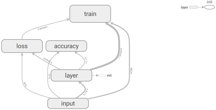
2.查看步骤：

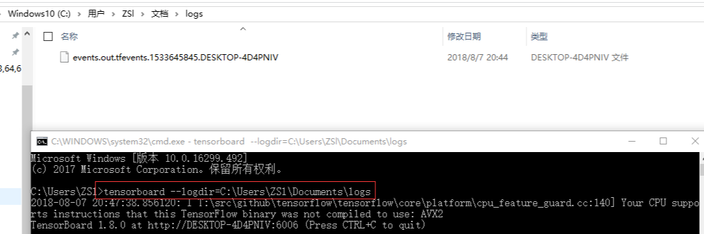
1.首先添加代码，将运行后的文件自动新建保存到log中

 write=tf.summary.FileWriter('logs/',sess.graph)#将图的结构存储在当前目录中

2.之后在所在文件的目录中（我的在C盘）通过命令提示符输入：tensorboard --logdir=C:\Users\ZSl\Documents\logs，然后把产生的Dos窗口中新的： http://DESKTOP-4D4PNIV:6006 地址复制用“谷歌”打开。显示如下图：

注意：

在添加不同的： with tf.name_scope('accuracy'): 时候，记得更新程序，重新执行Dos窗口，谷歌浏览器。
在Dos窗口重新执行时：“Ctrl+C”来在Dos中结束，并开始新的tensorboard --logdir=C:\Users\ZSl\Documents\logs
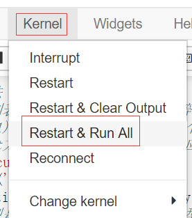
在Jupyter中，当重新执行时：之后（Restart&run all cells）。原因：只有这样，在tensorboard中生成的网络结构才不会保留上一次生成的网络。

tensorflow（8）tensorboard网络结构

猜你喜欢