R语言进行EDA ——ggplot 图形分面、直方图 和频率多边形

分面通常使用绘图方法+

①facet_wrap(~varible)/facet_wrap(formula)  较适用于单个变量

②facet_grid(vertical ~ horizion)/facet_grid(formula)  较适用于多个变量

详细讲解可参考 http://www.cookbook-r.com/Graphs/Facets_(ggplot2)/

其他图形调整

1、转换数据

### Transforming Data
Notes: 数据转换
```{r}
library(gridExtra) 
library(ggplot2)
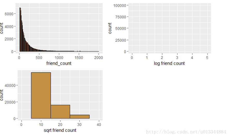
qplot(x=friend_count, data = pf)
summary(pf$friend_count)
summary(log10(pf$friend_count + 1))
summary(sqrt(pf$friend_count))

friend_count <- ggplot(aes(x = friend_count), data = pf) +
  geom_histogram(binwidth = 10, color = I("black"), fill = I("#F49045")) +
  scale_x_continuous(limits = c(0,2000))
friend_count_log <- ggplot(aes(x = log10(pf$friend_count+1)), data = pf) +
  geom_histogram(binwidth = 10, color = I("black"), fill = I("#C49045")) +
  scale_x_continuous(limits = c(0,5)) +
  xlab("log friend count")
friend_count_sqrt <- ggplot(aes(x = sqrt(pf$friend_count)), data = pf) +
  geom_histogram(binwidth = 10, color = I("black"), fill = I("#C49045")) +
  scale_x_continuous(limits = c(0,40)) +
  xlab("sqrt friend count")
grid.arrange(friend_count, friend_count_log, friend_count_sqrt, ncol = 2)


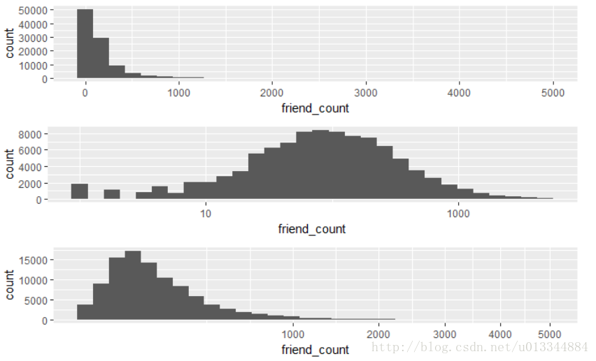
library(ggplot2)
p1 <- ggplot(aes(x = friend_count), data = pf) + geom_histogram()
p2 <- p1 + scale_x_log10() #log转换，qplot也可以这样做 ————标度层法
p3 <- p1 + scale_x_sqrt() # sqrt 转换
grid.arrange(p1,p2,p3,ncol=3)
```

在一个图像中输出多个图形方法：

首先下载程序包：

1	install.packages ( "gridExtra" )

然后定义不同的图形，并且arrange

1 2 3 4 5 6 7

# define individual plots p1 = ggplot (...) p2 = ggplot (...) p3 = ggplot (...) p4 = ggplot (...) # arrange plots in grid grid.arrange (p1, p2, p3, p4, ncol=2)

在一个图像输出内创建多个图形

向一个轴添加对数或 Sqrt 标尺

线性回归的假设

正态分布

在一个图中创建所有三个直方图之前，你需要运行以下代码： 

install.packages('gridExtra') 
library(gridExtra) 

数据的对数转换

2、频率多边形

```{r Frequency Polygons  error = TRUE, warning = FALSE}
#频率多边形 
qplot(x = friend_count, data = subset(pf,!is.na(gender)), binwidth=10) +
  scale_x_continuous(limits = c(0,1000), breaks = seq(0,1000,100)) +
  facet_wrap(~gender)

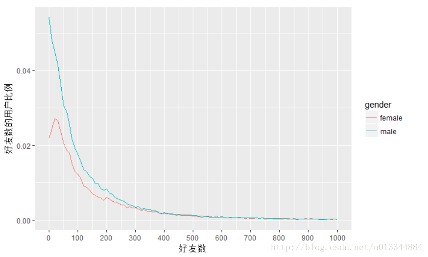
qplot(x = friend_count, y = ..count../sum(..count..), data = subset(pf,!is.na(gender)),
      xlab = "好友数", ylab = "好友数的用户比例",
      binwidth = 10, geom = "freqpoly", color = gender) +
  scale_x_continuous(limits = c(0,1000), breaks = seq(0,1000,100))

```

等效的 ggplot 语法： 
ggplot(aes(x = friend_count, y = ..count../sum(..count..)), data = subset(pf, !is.na(gender))) + 
  geom_freqpoly(aes(color = gender), binwidth=10) + 
  scale_x_continuous(limits = c(0, 1000), breaks = seq(0, 1000, 50)) + 
  xlab('好友数量') + 
  ylab('Percentage of users with that friend count')

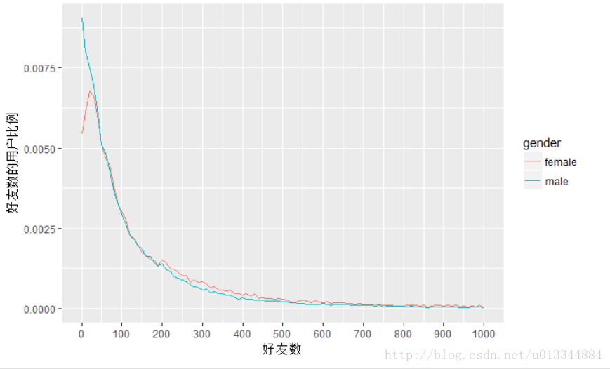
请注意，sum(..count..) 将跨颜色进行总计，因此，显示的百分比是总用户数的百分比。要在每个组内绘制百分比，你可以尝试

y = ..density...

用dengsity效果图

请注意，频率多边形的形状取决于我们如何设置箱子——在个别直方图中，线条的高度与条形的高度相同，但线条更容易进行比较，因为它们都在同一轴上。

等效的 ggplot 语法： 
ggplot(aes(x = www_likes), data = subset(pf, !is.na(gender))) + 
  geom_freqpoly(aes(color = gender)) + 
  scale_x_log10()

#根据gender分组总计www_likes
attach(pf)
by(www_likes, gender, sum)
detach(pf)