一、摘要
当环境奖励特别稀疏的时候,强化学习方法通常很难训练(traditionally struggle)。一个有效的方式是通过人类示范者(human demonstrator)提供模仿轨迹(imitate trajectories)来指导强化学习的探索方向,通常的做法是观看人类高手玩游戏的视频。
这里的问题是演示的素材(demonstrations),即人类高手的视频,通常不能直接使用。
因为不同的视频来源通常有细微的差异(domain gap),只有在完全相同的环境中(尺寸、分辨率、横纵比、颜色等等)获得状态信息\(S\),同时获得对应需要模仿的动作信息\(a\),甚至环境回报\(r\),然后构成状态动作对\((S,a)\)才能进行模仿学习。
比如,人类在观察一段游戏视频后,不管游戏是否存在色差、显示大小是否一样,都可以大致知道自己该如何操作(上下左右等),但是把这段视频提供给智能体(agent),微小的色差等显示变化都会让智能体误解成不同的状态,同时智能体也无法直接从视频中悟出该采取什么动作。归结起来就是两点:1. 游戏镜头不匹配(unaligned gameplay footage); 2. 没有动作标签(unlabeled)。
文章提出了一种分两步解决该问题的方法。1.通过自监督(self-supervised)的学习方式构造视频到状态抽象特征的映射,消除不同视频来源的细微差异造成的影响。2.用输出的抽象特征作为状态\(S\),结合模仿学习和强化学习探索最优动作。
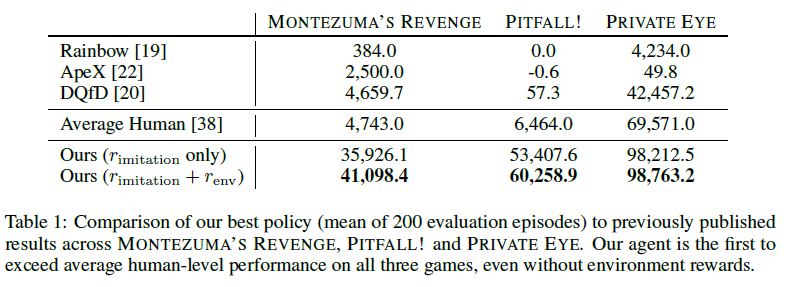
该方法在Montezuma's Revenge、Pitfall、Private Eye三个游戏中取得了超越人类水平的效果。
二、效果展示
- Montezuma's Revenge
- Pitfall
- Private Eye
三、具体问题和解决方法
1. Closing the domain gap
- 问题分析
这个问题(domain gap)就如摘要中所说,由于游戏存在不同版本,尺寸、分辨率、横纵比、颜色等等都有细微差别,所以就算是同一游戏状态,不同玩家的视频也不会完全匹配(unaligned footage)。如下图所示:
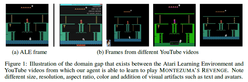
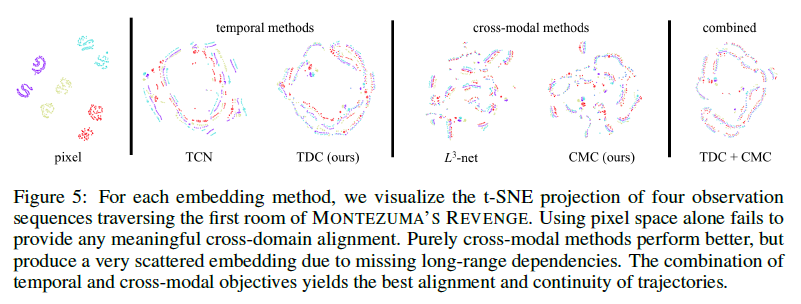
可以看到,对于同一游戏状态,右边四幅图在上述方面有明显的差异。本文提出的方法有效解决了这个问题。用t-SNE将处理后的特征可视化,效果如下图所示:
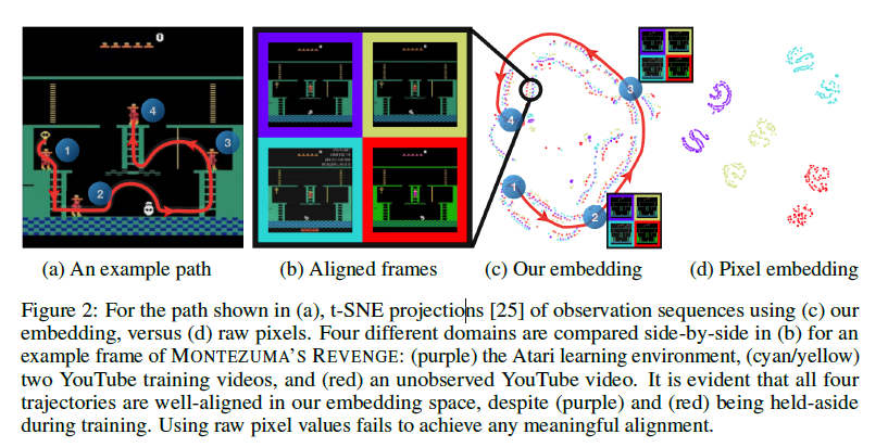
可以看到,通过该方法,不同来源的视频在特征空间上的表征一致,且可以和游戏动作序列化对应。 - 具体方法
对于这个问题,作者的想法是构造一个辅助任务让神经网络(embedding network)去学习,希望网络可以学到关键的特征而忽略不必要的差异。又由于没有任务标签,于是采用自监督(self-supervision)的方式构造标签并进行训练。文章提出了Temporal distance classification(TDC)和Cross-modal temporal distance classification(CMC)两种方法。- Temporal distance classification
利用同一视频中,视频序列的时间关系构建一个时间标签的监督学习任务,即让网络去预测同一视频中任意抽取的两帧图像之间的时间差分距离\(\Delta t\)。作者解释说,这个任务需要网络理解不同帧图像在时间上的转移关系,有助于网络学习到环境和agent交互过程中的环境变化规律(This task requires an understanding of how visual features move
and transform over time, thus encouraging an embedding that learns meaningful abstractions of
environment dynamics conditioned on agent interactions.)。
具体构造如下:
按照时间差分距离分成6个区间类别,记为\(d_k \in \{[0],[1],[2],[3-4],[5-20],[21-200]\}\)。其中[1]表示时间上相差1,[3-4]表示时间上相差3或者4,其他同理。考虑两帧图像\(v,w \in I\),我们让网络学会预测两帧图像的时间差区间\(d_k\)。具体的,这里构造了两个函数:visual embedding function \(\phi:I \rightarrow R^N\),classifier function \(\tau_{td}:R^N \times R^N \rightarrow R^K\)。其中visual embedding function从图像中提取出抽象特征(N维),classifier function预测两帧图像之间的时间差(K类的分类器)。每个函数都是一个神经网络,然后将两个网络合起来训练,即训练\(\tau_{td}(\phi(v),\phi(w))\)预测类别\(d_k\)。
损失函数使用交叉熵损失:
\(L_{td}(v^i,w^i,y^i)=-\sum_{j=1}^Ky_j^ilog(\hat{y}_j^i) \ \ \ with \ \ \hat{y}^i=\tau_{td}(\phi(v^i),\phi(w^i))\) 其中\(y^i\)为真实label,\(\hat{y}^i\)为网络预测的label。 - Cross-modal temporal distance classification
这种方法和前一种异曲同工,上述方法是在视频不同帧之间进行预测。该方法融入声音信息,将视频和声音进行匹配,预测两者之间的时间差,也就是所谓跨模态(cross-modal)的时间差分距离预测。作者解释说游戏的音频信息通常和动作事件高度相关,比如跳、捡到道具等等,这个任务有助于网络理解游戏中的重要事件(As the audio of Atari games tends to correspond with salient
events such as jumping, obtaining items or collecting points, a network that learns to correlate audio
and visual observations should learn an abstraction that emphasizes important game events.)。尽管在强化学习的游戏环境中没有声音信息,但结合音频信息构建embedding network有助于网络学习抽象特征。
具体构造如下:
视频数据(video frame)记为\(v \in I\),音频数据(audio snippet)记为\(a \in A\)。引入另一个音频特征提取的网络,audio embedding function \(\psi:A \rightarrow R^N\)。
损失函数同样为交叉熵损失:
\(L_{cm}(v^i,a^i,y^i)=-\sum_{j=1}^Ky_j^ilog(\hat{y}_j^i) \ \ \ with \ \ \ \hat{y}^i=\tau_{cm}(\phi(v^i),\psi(a^i))\)
- Temporal distance classification
- 结构设计
最终方法结合了TDC和CMC两种方法,设置权重\(\lambda\)计算综合损失:
\(L=L_{td}+\lambda L_{cm}\)
具体网络结构如下图:
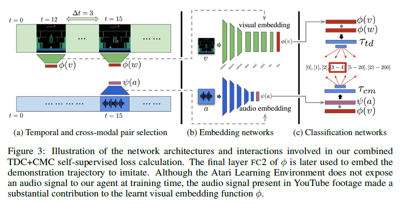
(a)图表示需要进行特征提取的原始数据,上面是视频数据,下面是音频数据。分别通过(b)图中的编码网络\(\phi(v)\)、\(\psi(a)\)提取主要特征并忽略无关的差异。最后将网络输入(c)图中的分类网络算出误差\(\tau_{td}\)和\(\tau_{cm}\),再反向传播训练网络。需要注意的是,这里\(\phi(v)\)和\(\psi(a)\)是两个独立不同的网络,\(\tau_{td}\)和\(\tau_{cm}\)网络结构相同,网络参数不同。
具体网络结构和训练数据生成的细节这里不是重点,直接粘贴原文:The visual embedding function \(\phi\)
The visual embedding function, \(\phi\), is composed of three spatial, padded, 3x3 convolutional layers
with (32, 64, 64) channels and 2x2 max-pooling, followed by three residual-connected blocks with
64 channels and no down-sampling. Each layer is ReLU-activated and batch-normalized, and the
output fed into a 2-layer 1024-wide MLP. The network input is a 128x128x3x4 tensor constructed
by random spatial cropping of a stack of four consecutive 140x140 RGB images, sampled from our
dataset. The final embedding vector is \(l_2\)-normalized.The audio embedding function \(\psi\)
The audio embedding function, \(\psi\) , is as per \(\phi\) except that it has four, width-8, 1D convolutional layers
with (32, 64, 128, 256) channels and 2x max-pooling, and a single width-1024 linear layer. The input
is a width-137 (6ms) sample of 256 frequency channels, calculated using STFT. ReLU-activation and
batch-normalization are applied throughout and the embedding vector is \(l_2\)-normalized.The classification network \(\tau\)
The same shallow network architecture, \(\tau\) , is used for both temporal and cross-modal classification.
Both input vectors are combined by element-wise multiplication, with the result fed into a 2-layer
MLP with widths (1024, 6) and ReLU non-linearity in between. A visualization of these networks and
their interaction is provided in Figure 3. Note that although \(\tau_{td}\) and \(\tau_{cm}\) share the same architecture,
they are operating on two different problems and therefore maintain separate sets of weights.Generating training data
To generate training data, we sample input pairs \((v_i,w_i)\) (where \(v_i\) and \(w_i\) are sampled from the
same domain) as follows. First, we sample a demonstration sequence from our three training videos.
Next, we sample both an interval, \(d_k \in {[0],[1],[2],[3-4],[5-20],[21-200]}\), and a distance,
\(\Delta t \in d_k\). Finally, we randomly select a pair of frames from the sequence with temporal distance \(\Delta t\).
The model is trained with Adam using a learning rate of \(10^{-4}\) and batch size of 32 for 200,000 steps.agent's network
As described in Section 4, our imitation loss is constructed by generating checkpoints every N = 16
frames along the \(\phi\)-embedded observation sequence of a single, held-aside YouTube video. We train
an agent using the sum of imitation and (optionally) environment rewards. We use the distributed
A3C RL agent IMPALA [14] with 100 actors for our experiments. The only modification we make to
the published network is to calculate the distance (as per Equation(2)) between the agent and the next
two checkpoints and concatenate this 2-vector with the flattened output of the last convolutional layer.
We also tried re-starting our agent from checkpoints recorded along its trajectory, similar to Hosu et
al. [23], but found that it provided minimal improvement given even our very long demonstrations.
- 效果评估
网络训练结束后,需要一种方式来评价编码网络的特征提取能力。受CycleGAN启发,作者提出了循环一致(cycle-consistency)评估方法。
假设有两段长度为\(N\)的序列片段\(V=\{v_1,v_2,...,v_n\}\)和\(W=\{w_1,w_2,...,w_n\}\)。在提取的特征空间上定义欧氏距离\(d_{\phi}\),\(d_{\phi}(v_i,w_j)=||\phi(v_i)-\phi(w_j)||_2\)。
评估方式如下:
— 先从\(V\)中挑选一帧数据\(v_i\),找出\(W\)中和\(v_i\)距离最近的一帧,\(w_j=\arg\min\limits_{w \in W}d_{\phi}(v_i,w)\)。
— 再从\(V\)中找出一帧和\(w_j\)距离最近的一帧,\(v_k=\arg\min\limits_{v \in V}d_{\phi}(v,w_j)\)。
— 如果\(v_i=v_k\),我们就称\(v_i\)是循环一致的(cycle-consistency)。
— 同时再定义一个一一对应的特征匹配能力的指标,记为\(P_{\phi}\)。\(P_{\phi}\)表示在特征空间\(\phi\)上特征数据\(v \in V\)是循环一致(cycle-consistent)的百分比。
此外,根据定义也可以在\(\phi\)上定义三重循环一致(3-cycle-consistency)和匹配能力指标\(P_{\phi}^3\)。这要求\(v_i\)在三个序列\(V,W,U\)上满足\(V \rightarrow W \rightarrow U \rightarrow V\)和\(V \rightarrow U \rightarrow W \rightarrow V\)。
实验效果如下:
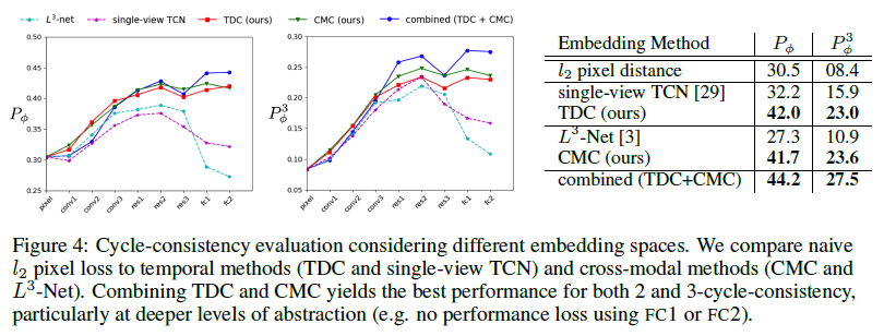
可以看到TDC+CMC的效果是最好的。用t-SNE可视化展示如下:
2. One-shot imitation from YouTube footage
- 问题分析
domain gap问题已经解决,接下来是如何利用数据进行训练。目前已经将游戏视频和agent的环境状态对应上,但依然没有动作和回报信息。作者选择了其中一个视频(a single YouTube gameplay video)根据状态序列让网络学习。也就是说前面训练特征提取的网络时,使用了多个视频,这里模仿学习只用了一个视频。按照作者的意思,一共有四个视频,用三个视频训练特征提取网络,用另一个视频让agent学习。 - 具体方法
学习思路是让agent在环境中探索动作,如果得到的状态和视频的状态匹配,说明模仿到位,给一个大于0的回报,否则不给回报,也不给惩罚。具体学习方法如下:
对于该视频,每隔\(N\)帧(\(N=16\))设置一个检查点(checkpoint),设置模仿回报
\[ r_{imitation}=\left\{\begin{array}{l}0.5 \ \ \ \ \ if \ \ \bar{\phi}(v_{agent})\cdot \bar{\phi}(v_{checkpoint})>\gamma \\0.0\ \ \ \ \ otherwise\end{array}\right.\]
其中\(\gamma\)是衡量匹配度的阈值,\(\bar{\phi}(v)\)经过均值方差归一化(zero-centered and \(l_2\)-normalized),所以可以通过向量点乘的方式度量匹配度。
需要注意的是,模仿的动作不必完全一样,允许网络有自己的探索,所以文章把检查点(checkpoint)设置成软顺序(soft-order)。具体说来,当上一步的checkpoint和\(v^{(n)}\)匹配时,下一个checkpoint不用必须和\(v^{(n+1)}\)匹配,只要下一个checkpoint和\(\Delta t\)时间内的状态相匹配就给予奖励,即只需要\(v_{checkpoint} \in \{v^{n+1},..,v^{n+1+\Delta t}\}\)。文中的设置为\(\Delta t =1,\gamma=0.5\),当只有图像特征没有音频时,设置\(\gamma=0.92\)效果更好。
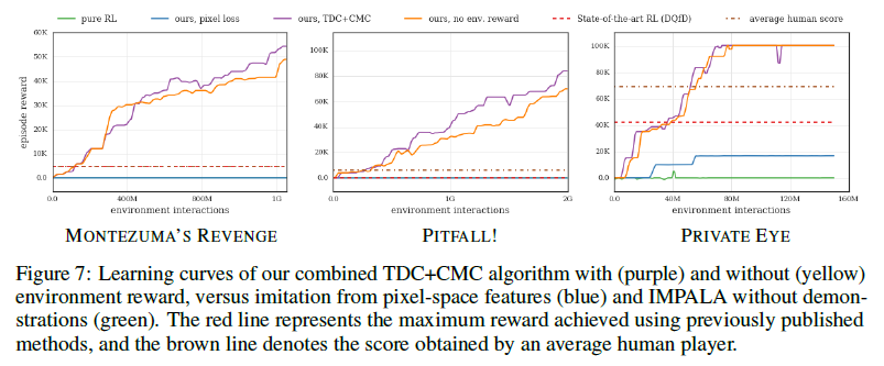
训练方法上,直接使用传统的强化学习算法:分布式的A3C算法(distributed A3C RL agent IMPALA)。一共使用100个actor,reward设置为模仿学习的reward:\(r_{imitation}\),或者模仿学习reward和游戏reward之和:\(r_{imitation}+r_{game}\)。这样就得到了开头视频的展示效果。
到此,方法介绍完毕。
四、实验结果
作者在文中给出了一些实验数据,主要有特征提取的效果度量,和模仿学习的曲线以及游戏得分。
- one-to-one alignment capacity
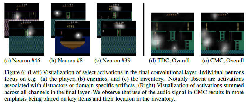
- meaningful abstraction
- learning curves
- score
五、总结
这篇文章确实在三个游戏上做出了效果,这毋庸置疑,但得分超过人类水平的主要原因还是在于模仿了人类高手的玩法。其创新不在于强化学习的算法,主要在于如何直接从视频源进行模仿学习,避开了匹配状态动作对\((S,a)\)的数据预处理步骤。关键点在于构造辅助任务,训练特征提取网络,更多的可以看做是一篇CV的文章。
不过将模仿学习和强化学习相结合的训练方式,值得认真思考和研究。