Deep Learning with TensorFlow
IBM Cognitive Class ML0120EN
Module 5 - Autoencoders

使用DBN识别手写体
传统的多层感知机或者神经网络的一个问题：反向传播可能总是导致局部最小值。
当误差表面(error surface)包含了多个凹槽，当你做梯度下降时，你找到的并不是最深的凹槽。下面你将会看到DBN是怎么解决这个问题的。

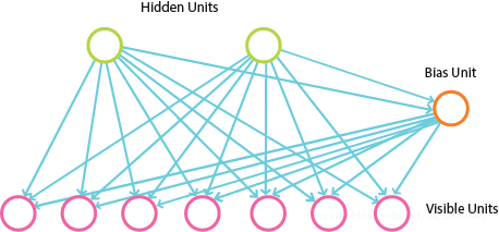
深度置信网络

深度置信网络可以通过额外的预训练规程解决局部最小值的问题。预训练在反向传播之前做完，这样可以使错误率离最优的解不是那么远，也就是我们在最优解的附近。再通过反向传播慢慢地降低错误率。
深度置信网络主要分成两部分。第一部分是多层玻尔兹曼感知机，用于预训练我们的网络。第二部分是前馈反向传播网络，这可以使RBM堆叠的网络更加精细化。

1. 加载必要的深度置信网络库

#urllib is used to download the utils file from deeplearning.net
import urllib
response = urllib.urlopen('http://deeplearning.net/tutorial/code/utils.py')
content = response.read()
target = open('utils.py', 'w')
target.write(content)
target.close()
#Import the math function for calculations
import math
#Tensorflow library. Used to implement machine learning models
import tensorflow as tf
#Numpy contains helpful functions for efficient mathematical calculations
import numpy as np
#Image library for image manipulation
from PIL import Image
#import Image
#Utils file
from utils import tile_raster_images

2. 构建RBM层

RBM的细节参考【这里】
rbm
为了在Tensorflow中应用DBM, 下面创建一个RBM的类

#Class that defines the behavior of the RBM
class RBM(object):

    def __init__(self, input_size, output_size):
        #Defining the hyperparameters
        self._input_size = input_size #Size of input
        self._output_size = output_size #Size of output
        self.epochs = 5 #Amount of training iterations
        self.learning_rate = 1.0 #The step used in gradient descent
        self.batchsize = 100 #The size of how much data will be used for training per sub iteration

        #Initializing weights and biases as matrices full of zeroes
        self.w = np.zeros([input_size, output_size], np.float32) #Creates and initializes the weights with 0
        self.hb = np.zeros([output_size], np.float32) #Creates and initializes the hidden biases with 0
        self.vb = np.zeros([input_size], np.float32) #Creates and initializes the visible biases with 0


    #Fits the result from the weighted visible layer plus the bias into a sigmoid curve
    def prob_h_given_v(self, visible, w, hb):
        #Sigmoid 
        return tf.nn.sigmoid(tf.matmul(visible, w) + hb)

    #Fits the result from the weighted hidden layer plus the bias into a sigmoid curve
    def prob_v_given_h(self, hidden, w, vb):
        return tf.nn.sigmoid(tf.matmul(hidden, tf.transpose(w)) + vb)

    #Generate the sample probability
    def sample_prob(self, probs):
        return tf.nn.relu(tf.sign(probs - tf.random_uniform(tf.shape(probs))))

    #Training method for the model
    def train(self, X):
        #Create the placeholders for our parameters
        _w = tf.placeholder("float", [self._input_size, self._output_size])
        _hb = tf.placeholder("float", [self._output_size])
        _vb = tf.placeholder("float", [self._input_size])

        prv_w = np.zeros([self._input_size, self._output_size], np.float32) #Creates and initializes the weights with 0
        prv_hb = np.zeros([self._output_size], np.float32) #Creates and initializes the hidden biases with 0
        prv_vb = np.zeros([self._input_size], np.float32) #Creates and initializes the visible biases with 0


        cur_w = np.zeros([self._input_size, self._output_size], np.float32)
        cur_hb = np.zeros([self._output_size], np.float32)
        cur_vb = np.zeros([self._input_size], np.float32)
        v0 = tf.placeholder("float", [None, self._input_size])

        #Initialize with sample probabilities
        h0 = self.sample_prob(self.prob_h_given_v(v0, _w, _hb))
        v1 = self.sample_prob(self.prob_v_given_h(h0, _w, _vb))
        h1 = self.prob_h_given_v(v1, _w, _hb)

        #Create the Gradients
        positive_grad = tf.matmul(tf.transpose(v0), h0)
        negative_grad = tf.matmul(tf.transpose(v1), h1)

        #Update learning rates for the layers
        update_w = _w + self.learning_rate *(positive_grad - negative_grad) / tf.to_float(tf.shape(v0)[0])
        update_vb = _vb +  self.learning_rate * tf.reduce_mean(v0 - v1, 0)
        update_hb = _hb +  self.learning_rate * tf.reduce_mean(h0 - h1, 0)

        #Find the error rate
        err = tf.reduce_mean(tf.square(v0 - v1))

        #Training loop
        with tf.Session() as sess:
            sess.run(tf.initialize_all_variables())
            #For each epoch
            for epoch in range(self.epochs):
                #For each step/batch
                for start, end in zip(range(0, len(X), self.batchsize),range(self.batchsize,len(X), self.batchsize)):
                    batch = X[start:end]
                    #Update the rates
                    cur_w = sess.run(update_w, feed_dict={v0: batch, _w: prv_w, _hb: prv_hb, _vb: prv_vb})
                    cur_hb = sess.run(update_hb, feed_dict={v0: batch, _w: prv_w, _hb: prv_hb, _vb: prv_vb})
                    cur_vb = sess.run(update_vb, feed_dict={v0: batch, _w: prv_w, _hb: prv_hb, _vb: prv_vb})
                    prv_w = cur_w
                    prv_hb = cur_hb
                    prv_vb = cur_vb
                error=sess.run(err, feed_dict={v0: X, _w: cur_w, _vb: cur_vb, _hb: cur_hb})
                print 'Epoch: %d' % epoch,'reconstruction error: %f' % error
            self.w = prv_w
            self.hb = prv_hb
            self.vb = prv_vb

    #Create expected output for our DBN
    def rbm_outpt(self, X):
        input_X = tf.constant(X)
        _w = tf.constant(self.w)
        _hb = tf.constant(self.hb)
        out = tf.nn.sigmoid(tf.matmul(input_X, _w) + _hb)
        with tf.Session() as sess:
            sess.run(tf.global_variables_initializer())
            return sess.run(out)

3. 导入MNIST数据

使用one-hot encoding标注的形式载入MNIST图像数据。

#Getting the MNIST data provided by Tensorflow
from tensorflow.examples.tutorials.mnist import input_data

#Loading in the mnist data
mnist = input_data.read_data_sets("MNIST_data/", one_hot=True)
trX, trY, teX, teY = mnist.train.images, mnist.train.labels, mnist.test.images,\
    mnist.test.labels


Extracting MNIST_data/train-images-idx3-ubyte.gz
Extracting MNIST_data/train-labels-idx1-ubyte.gz
Extracting MNIST_data/t10k-images-idx3-ubyte.gz
Extracting MNIST_data/t10k-labels-idx1-ubyte.gz

4. 建立DBN

RBM_hidden_sizes = [500, 200 , 50 ] #create 2 layers of RBM with size 400 and 100

#Since we are training, set input as training data
inpX = trX

#Create list to hold our RBMs
rbm_list = []

#Size of inputs is the number of inputs in the training set
input_size = inpX.shape[1]

#For each RBM we want to generate
for i, size in enumerate(RBM_hidden_sizes):
    print 'RBM: ',i,' ',input_size,'->', size
    rbm_list.append(RBM(input_size, size))
    input_size = size

RBM:  0   784 -> 500
RBM:  1   500 -> 200
RBM:  2   200 -> 50

rbm的类创建好了和数据都已经载入，可以创建DBN。在这个例子中，我们使用了3个RBM，一个的隐藏层单元个数为500，第二个RBM的隐藏层个数为200，最后一个为50. 我们想要生成训练数据的深层次表示形式。

5.训练RBM

我们将使用rbm.train()开始预训练步骤, 单独训练堆中的每一个RBM，并将当前RBM的输出作为下一个RBM的输入。

#For each RBM in our list
for rbm in rbm_list:
    print 'New RBM:'
    #Train a new one
    rbm.train(inpX) 
    #Return the output layer
    inpX = rbm.rbm_outpt(inpX)

New RBM:
Epoch: 0 reconstruction error: 0.061884
Epoch: 1 reconstruction error: 0.052996
Epoch: 2 reconstruction error: 0.049414
Epoch: 3 reconstruction error: 0.047123
Epoch: 4 reconstruction error: 0.046149
New RBM:
Epoch: 0 reconstruction error: 0.035305
Epoch: 1 reconstruction error: 0.031168
Epoch: 2 reconstruction error: 0.029394
Epoch: 3 reconstruction error: 0.028474
Epoch: 4 reconstruction error: 0.027456
New RBM:
Epoch: 0 reconstruction error: 0.055896
Epoch: 1 reconstruction error: 0.053111
Epoch: 2 reconstruction error: 0.051631
Epoch: 3 reconstruction error: 0.051126
Epoch: 4 reconstruction error: 0.051245

现在我们可以将输入数据的学习好的表示转换为有监督的预测，比如一个线性分类器。特别地，我们使用这个浅层神经网络的最后一层的输出对数字分类。

6. 神经网络

下面的类使用了上面预训练好的RBMs实现神经网络。

import numpy as np
import math
import tensorflow as tf


class NN(object):

    def __init__(self, sizes, X, Y):
        #Initialize hyperparameters
        self._sizes = sizes
        self._X = X
        self._Y = Y
        self.w_list = []
        self.b_list = []
        self._learning_rate =  1.0
        self._momentum = 0.0
        self._epoches = 10
        self._batchsize = 100
        input_size = X.shape[1]

        #initialization loop
        for size in self._sizes + [Y.shape[1]]:
            #Define upper limit for the uniform distribution range
            max_range = 4 * math.sqrt(6. / (input_size + size))

            #Initialize weights through a random uniform distribution
            self.w_list.append(
                np.random.uniform( -max_range, max_range, [input_size, size]).astype(np.float32))

            #Initialize bias as zeroes
            self.b_list.append(np.zeros([size], np.float32))
            input_size = size

    #load data from rbm
    def load_from_rbms(self, dbn_sizes,rbm_list):
        #Check if expected sizes are correct
        assert len(dbn_sizes) == len(self._sizes)

        for i in range(len(self._sizes)):
            #Check if for each RBN the expected sizes are correct
            assert dbn_sizes[i] == self._sizes[i]

        #If everything is correct, bring over the weights and biases
        for i in range(len(self._sizes)):
            self.w_list[i] = rbm_list[i].w
            self.b_list[i] = rbm_list[i].hb

    #Training method
    def train(self):
        #Create placeholders for input, weights, biases, output
        _a = [None] * (len(self._sizes) + 2)
        _w = [None] * (len(self._sizes) + 1)
        _b = [None] * (len(self._sizes) + 1)
        _a[0] = tf.placeholder("float", [None, self._X.shape[1]])
        y = tf.placeholder("float", [None, self._Y.shape[1]])

        #Define variables and activation functoin
        for i in range(len(self._sizes) + 1):
            _w[i] = tf.Variable(self.w_list[i])
            _b[i] = tf.Variable(self.b_list[i])
        for i in range(1, len(self._sizes) + 2):
            _a[i] = tf.nn.sigmoid(tf.matmul(_a[i - 1], _w[i - 1]) + _b[i - 1])

        #Define the cost function
        cost = tf.reduce_mean(tf.square(_a[-1] - y))

        #Define the training operation (Momentum Optimizer minimizing the Cost function)
        train_op = tf.train.MomentumOptimizer(
            self._learning_rate, self._momentum).minimize(cost)

        #Prediction operation
        predict_op = tf.argmax(_a[-1], 1)

        #Training Loop
        with tf.Session() as sess:
            #Initialize Variables
            sess.run(tf.global_variables_initializer())

            #For each epoch
            for i in range(self._epoches):

                #For each step
                for start, end in zip(
                    range(0, len(self._X), self._batchsize), range(self._batchsize, len(self._X), self._batchsize)):

                    #Run the training operation on the input data
                    sess.run(train_op, feed_dict={
                        _a[0]: self._X[start:end], y: self._Y[start:end]})

                for j in range(len(self._sizes) + 1):
                    #Retrieve weights and biases
                    self.w_list[j] = sess.run(_w[j])
                    self.b_list[j] = sess.run(_b[j])

                print "Accuracy rating for epoch " + str(i) + ": " + str(np.mean(np.argmax(self._Y, axis=1) ==
                              sess.run(predict_op, feed_dict={_a[0]: self._X, y: self._Y})))

7. 运行

nNet = NN(RBM_hidden_sizes, trX, trY)
nNet.load_from_rbms(RBM_hidden_sizes,rbm_list)
nNet.train()

Accuracy rating for epoch 0: 0.39641818181818184
Accuracy rating for epoch 1: 0.664309090909091
Accuracy rating for epoch 2: 0.7934545454545454
Accuracy rating for epoch 3: 0.8152727272727273
Accuracy rating for epoch 4: 0.8258181818181818
Accuracy rating for epoch 5: 0.8348727272727273
Accuracy rating for epoch 6: 0.8525272727272727
Accuracy rating for epoch 7: 0.889109090909091
Accuracy rating for epoch 8: 0.9079454545454545
Accuracy rating for epoch 9: 0.9158

参考文献

• http://deeplearning.net/tutorial/DBN.html
• https://github.com/myme5261314/dbn_tf

本文译自： ML0120EN-5.2-Review-DBNMNIST.ipynb