工具系列：TensorFlow决策森林_(8)组合决策森林和神经网络模型

文章目录

介绍

欢迎来到TensorFlow Decision Forests（TF-DF）的模型组合教程。本教程将向您展示如何使用通用的预处理层和Keras函数式API将多个决策森林和神经网络模型组合在一起。

您可能希望将模型组合在一起以提高预测性能（集成），以获得不同建模技术的最佳效果（异构模型集成），在不同数据集上训练模型的不同部分（例如预训练），或创建堆叠模型（例如，一个模型在另一个模型的预测上操作）。

本教程涵盖了使用函数式API进行模型组合的高级用例。您可以在本教程的“特征预处理”部分和本教程的“使用预训练文本嵌入”部分中找到更简单的模型组合场景的示例。

以下是您将构建的模型的结构：

# 安装graphviz库
!pip install graphviz -U --quiet

# 导入graphviz库中的Source类
from graphviz import Source

# 创建一个Source对象，传入一个字符串表示的dot语言图形描述
Source("""
digraph G {
  raw_data [label="Input features"];  # 创建一个节点，表示原始数据
  preprocess_data [label="Learnable NN pre-processing", shape=rect];  # 创建一个节点，表示可学习的神经网络预处理

  raw_data -> preprocess_data  # 原始数据指向神经网络预处理节点

  subgraph cluster_0 {
    color=grey;
    a1[label="NN layer", shape=rect];  # 创建一个节点，表示神经网络层
    b1[label="NN layer", shape=rect];  # 创建一个节点，表示神经网络层
    a1 -> b1;  # 神经网络层之间的连接
	label = "Model #1";  # 设置子图的标签为"Model #1"
  }

   subgraph cluster_1 {
    color=grey;
    a2[label="NN layer", shape=rect];  # 创建一个节点，表示神经网络层
    b2[label="NN layer", shape=rect];  # 创建一个节点，表示神经网络层
    a2 -> b2;  # 神经网络层之间的连接
	label = "Model #2";  # 设置子图的标签为"Model #2"
  }

  subgraph cluster_2 {
    color=grey;
    a3[label="Decision Forest", shape=rect];  # 创建一个节点，表示决策森林
	label = "Model #3";  # 设置子图的标签为"Model #3"
  }

  subgraph cluster_3 {
    color=grey;
    a4[label="Decision Forest", shape=rect];  # 创建一个节点，表示决策森林
	label = "Model #4";  # 设置子图的标签为"Model #4"
  }

  preprocess_data -> a1;  # 神经网络预处理节点指向神经网络层节点
  preprocess_data -> a2;  # 神经网络预处理节点指向神经网络层节点
  preprocess_data -> a3;  # 神经网络预处理节点指向决策森林节点
  preprocess_data -> a4;  # 神经网络预处理节点指向决策森林节点

  b1  -> aggr;  # 神经网络层节点指向聚合节点
  b2  -> aggr;  # 神经网络层节点指向聚合节点
  a3 -> aggr;  # 决策森林节点指向聚合节点
  a4 -> aggr;  # 决策森林节点指向聚合节点

  aggr [label="Aggregation (mean)", shape=rect]  # 创建一个节点，表示聚合操作（平均值）
  aggr -> predictions  # 聚合节点指向预测结果节点
}
""")

在这里插入图片描述

你的组合模型有三个阶段：

第一阶段是一个预处理层，由神经网络组成，对下一阶段的所有模型都是共同的。在实践中，这样的预处理层可以是一个预训练的嵌入层进行微调，也可以是一个随机初始化的神经网络。
第二阶段是两个决策森林和两个神经网络模型的集合。
最后一个阶段是对第二阶段模型的预测进行平均。它不包含任何可学习的权重。

神经网络使用反向传播算法和梯度下降进行训练。该算法具有两个重要特性：(1)如果神经网络层接收到损失梯度(更精确地说，是根据该层的输出计算的损失梯度)，则该层可以进行训练；(2)该算法将损失梯度从层的输出“传递”到层的输入(这是“链式法则”)。由于这两个原因，反向传播可以同时训练多层神经网络堆叠在一起。

在这个例子中，决策森林是使用随机森林(RF)算法进行训练的。与反向传播不同，RF的训练不会将损失梯度从其输出传递到其输入。因此，传统的RF算法不能用于训练或微调神经网络。换句话说，“决策森林”阶段不能用于训练“可学习的NN预处理块”。

训练预处理和神经网络阶段。
训练决策森林阶段。

安装 TensorFlow Decision Forests

通过运行以下单元格来安装 TF-DF。

!pip install tensorflow_decision_forests -U --quiet

Wurlitzer 是在Colabs中显示详细的训练日志所需的（当在模型构造函数中使用verbose=2时）。

# 安装wurlitzer库，用于在Jupyter Notebook中显示命令行输出信息
!pip install wurlitzer -U --quiet

导入库

# 导入所需的库

# 导入tensorflow_decision_forests库
import tensorflow_decision_forests as tfdf

# 导入其他库
import os
import numpy as np
import pandas as pd
import tensorflow as tf
import math
import matplotlib.pyplot as plt

数据集

在本教程中，您将使用一个简单的合成数据集，以便更容易解释最终的模型。

# 定义函数make_dataset，用于生成数据集
# 参数：
#   - num_examples: 数据集中的样本数量
#   - num_features: 每个样本的特征数量
#   - seed: 随机种子，用于生成随机数
# 返回值：
#   - features: 生成的特征矩阵，形状为(num_examples, num_features)
#   - labels: 生成的标签矩阵，形状为(num_examples,)

def make_dataset(num_examples, num_features, seed=1234):
    # 设置随机种子
    np.random.seed(seed)
    
    # 生成特征矩阵，形状为(num_examples, num_features)
    features = np.random.uniform(-1, 1, size=(num_examples, num_features))
    
    # 生成噪声矩阵，形状为(num_examples,)
    noise = np.random.uniform(size=(num_examples))
    
    # 计算左侧部分
    left_side = np.sqrt(
        np.sum(np.multiply(np.square(features[:, 0:2]), [1, 2]), axis=1))
    
    # 计算右侧部分
    right_side = features[:, 2] * 0.7 + np.sin(
        features[:, 3] * 10) * 0.5 + noise * 0.0 + 0.5
    
    # 根据左侧和右侧的大小关系，生成标签矩阵
    labels = left_side <= right_side
    
    # 将标签矩阵转换为整数类型，并返回特征矩阵和标签矩阵
    return features, labels.astype(int)

生成一些示例：

make_dataset(num_examples=5, num_features=4)

(array([[-0.6169611 ,  0.24421754, -0.12454452,  0.57071717],
        [ 0.55995162, -0.45481479, -0.44707149,  0.60374436],
        [ 0.91627871,  0.75186527, -0.28436546,  0.00199025],
        [ 0.36692587,  0.42540405, -0.25949849,  0.12239237],
        [ 0.00616633, -0.9724631 ,  0.54565324,  0.76528238]]),
 array([0, 0, 0, 1, 0]))

您还可以绘制它们以了解合成模式的大致情况：

# 生成数据集
plot_features, plot_label = make_dataset(num_examples=50000, num_features=4)

# 设置图形大小
plt.rcParams["figure.figsize"] = [8, 8]

# 设置散点图的公共参数
common_args = dict(c=plot_label, s=1.0, alpha=0.5)

# 创建子图1，并绘制散点图
plt.subplot(2, 2, 1)
plt.scatter(plot_features[:, 0], plot_features[:, 1], **common_args)

# 创建子图2，并绘制散点图
plt.subplot(2, 2, 2)
plt.scatter(plot_features[:, 1], plot_features[:, 2], **common_args)

# 创建子图3，并绘制散点图
plt.subplot(2, 2, 3)
plt.scatter(plot_features[:, 0], plot_features[:, 2], **common_args)

# 创建子图4，并绘制散点图
plt.subplot(2, 2, 4)
plt.scatter(plot_features[:, 0], plot_features[:, 3], **common_args)

<matplotlib.collections.PathCollection at 0x7fad984548e0>

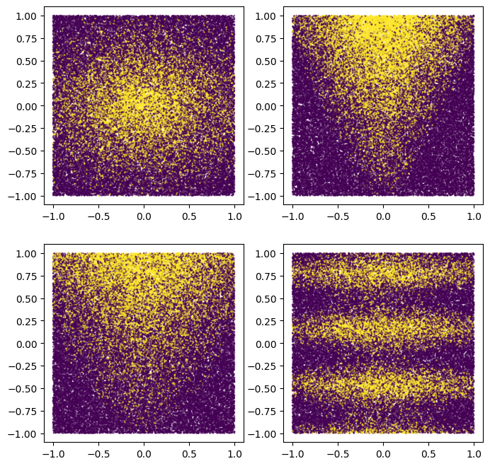
请注意，这种模式是平滑的，而且不是轴对齐的。这将有利于神经网络模型。这是因为对于神经网络来说，拥有圆形和非对齐的决策边界比决策树更容易。

另一方面，我们将在一个包含2500个示例的小数据集上训练模型。这将有利于决策森林模型。这是因为决策森林更加高效，能够利用所有可用的示例信息（决策森林具有“样本高效性”）。

我们的神经网络和决策森林集成将兼具两者的优点。

让我们创建一个训练和测试的tf.data.Dataset：

# 定义函数make_tf_dataset，参数为batch_size和其他参数
def make_tf_dataset(batch_size=64, **args):
  # 调用make_dataset函数，返回features和labels
  features, labels = make_dataset(**args)
  # 使用tf.data.Dataset.from_tensor_slices将features和labels转换为Dataset类型，并按batch_size划分batch
  return tf.data.Dataset.from_tensor_slices(
      (features, labels)).batch(batch_size)

# 定义变量num_features为10

# 调用make_tf_dataset函数，生成训练集train_dataset，包含2500个样本，每个样本包含num_features个特征，每个batch包含100个样本，随机数种子为1234
train_dataset = make_tf_dataset(
    num_examples=2500, num_features=num_features, batch_size=100, seed=1234)

# 调用make_tf_dataset函数，生成测试集test_dataset，包含10000个样本，每个样本包含num_features个特征，每个batch包含100个样本，随机数种子为5678
test_dataset = make_tf_dataset(
    num_examples=10000, num_features=num_features, batch_size=100, seed=5678)

模型结构

将模型结构定义如下：

# 输入特征
raw_features = tf.keras.layers.Input(shape=(num_features,))

# 阶段1
# =======

# 公共可学习的预处理
preprocessor = tf.keras.layers.Dense(10, activation=tf.nn.relu6)
preprocess_features = preprocessor(raw_features)

# 阶段2
# =======

# 模型1：神经网络
m1_z1 = tf.keras.layers.Dense(5, activation=tf.nn.relu6)(preprocess_features)
m1_pred = tf.keras.layers.Dense(1, activation=tf.nn.sigmoid)(m1_z1)

# 模型2：神经网络
m2_z1 = tf.keras.layers.Dense(5, activation=tf.nn.relu6)(preprocess_features)
m2_pred = tf.keras.layers.Dense(1, activation=tf.nn.sigmoid)(m2_z1)


# 模型3：决策树随机森林
model_3 = tfdf.keras.RandomForestModel(num_trees=1000, random_seed=1234)
m3_pred = model_3(preprocess_features)

# 模型4：决策树随机森林
model_4 = tfdf.keras.RandomForestModel(
    num_trees=1000,
    #split_axis="SPARSE_OBLIQUE", # 取消注释此行以提高该模型的质量
    random_seed=4567)
m4_pred = model_4(preprocess_features)

# 由于TF-DF使用确定性学习算法，您应该将模型的训练种子设置为不同的值，否则两个`tfdf.keras.RandomForestModel`将完全相同。

# 阶段3
# =======

mean_nn_only = tf.reduce_mean(tf.stack([m1_pred, m2_pred], axis=0), axis=0)
mean_nn_and_df = tf.reduce_mean(
    tf.stack([m1_pred, m2_pred, m3_pred, m4_pred], axis=0), axis=0)

# Keras模型
# ============

ensemble_nn_only = tf.keras.models.Model(raw_features, mean_nn_only)
ensemble_nn_and_df = tf.keras.models.Model(raw_features, mean_nn_and_df)

Warning: The `num_threads` constructor argument is not set and the number of CPU is os.cpu_count()=32 > 32. Setting num_threads to 32. Set num_threads manually to use more than 32 cpus.


WARNING:absl:The `num_threads` constructor argument is not set and the number of CPU is os.cpu_count()=32 > 32. Setting num_threads to 32. Set num_threads manually to use more than 32 cpus.


Use /tmpfs/tmp/tmpeqn1u3t4 as temporary training directory
Warning: The model was called directly (i.e. using `model(data)` instead of using `model.predict(data)`) before being trained. The model will only return zeros until trained. The output shape might change after training Tensor("inputs:0", shape=(None, 10), dtype=float32)


WARNING:absl:The model was called directly (i.e. using `model(data)` instead of using `model.predict(data)`) before being trained. The model will only return zeros until trained. The output shape might change after training Tensor("inputs:0", shape=(None, 10), dtype=float32)


Warning: The `num_threads` constructor argument is not set and the number of CPU is os.cpu_count()=32 > 32. Setting num_threads to 32. Set num_threads manually to use more than 32 cpus.


WARNING:absl:The `num_threads` constructor argument is not set and the number of CPU is os.cpu_count()=32 > 32. Setting num_threads to 32. Set num_threads manually to use more than 32 cpus.


Use /tmpfs/tmp/tmpzrq7x74t as temporary training directory
Warning: The model was called directly (i.e. using `model(data)` instead of using `model.predict(data)`) before being trained. The model will only return zeros until trained. The output shape might change after training Tensor("inputs:0", shape=(None, 10), dtype=float32)


WARNING:absl:The model was called directly (i.e. using `model(data)` instead of using `model.predict(data)`) before being trained. The model will only return zeros until trained. The output shape might change after training Tensor("inputs:0", shape=(None, 10), dtype=float32)

在训练模型之前，您可以绘制它以检查它是否与初始图表相似。

# 导入plot_model函数
from keras.utils import plot_model

# 使用plot_model函数将模型ensemble_nn_and_df可视化，并保存为图片
# 参数to_file指定保存的文件路径为/tmp/model.png
# 参数show_shapes设置为True，表示在可视化图中显示每个层的输入输出形状
plot_model(ensemble_nn_and_df, to_file="/tmp/model.png", show_shapes=True)

模型训练

首先使用反向传播算法训练预处理和两个神经网络层。

%%time
# 编译模型
ensemble_nn_only.compile(
    optimizer=tf.keras.optimizers.Adam(),  # 使用Adam优化器来优化模型的参数
    loss=tf.keras.losses.BinaryCrossentropy(),  # 使用二元交叉熵作为损失函数
    metrics=["accuracy"]  # 使用准确率作为评估指标
)

# 训练模型
ensemble_nn_only.fit(
    train_dataset,  # 使用训练数据集进行训练
    epochs=20,  # 迭代20次
    validation_data=test_dataset  # 使用测试数据集进行验证
)

Epoch 1/20

 1/25 [>.............................] - ETA: 1:49 - loss: 0.5916 - accuracy: 0.7200
18/25 [====================>.........] - ETA: 0s - loss: 0.5695 - accuracy: 0.7556  
25/25 [==============================] - 5s 15ms/step - loss: 0.5691 - accuracy: 0.7500 - val_loss: 0.5662 - val_accuracy: 0.7392
Epoch 2/20

 1/25 [>.............................] - ETA: 0s - loss: 0.5743 - accuracy: 0.7200
19/25 [=====================>........] - ETA: 0s - loss: 0.5510 - accuracy: 0.7574
25/25 [==============================] - 0s 9ms/step - loss: 0.5542 - accuracy: 0.7500 - val_loss: 0.5554 - val_accuracy: 0.7392
Epoch 3/20

 1/25 [>.............................] - ETA: 0s - loss: 0.5623 - accuracy: 0.7200
19/25 [=====================>........] - ETA: 0s - loss: 0.5396 - accuracy: 0.7574
25/25 [==============================] - 0s 9ms/step - loss: 0.5434 - accuracy: 0.7500 - val_loss: 0.5467 - val_accuracy: 0.7392
Epoch 4/20

 1/25 [>.............................] - ETA: 0s - loss: 0.5525 - accuracy: 0.7200
17/25 [===================>..........] - ETA: 0s - loss: 0.5362 - accuracy: 0.7529
25/25 [==============================] - 0s 10ms/step - loss: 0.5342 - accuracy: 0.7500 - val_loss: 0.5384 - val_accuracy: 0.7392
Epoch 5/20

 1/25 [>.............................] - ETA: 0s - loss: 0.5433 - accuracy: 0.7200
18/25 [====================>.........] - ETA: 0s - loss: 0.5244 - accuracy: 0.7556
25/25 [==============================] - 0s 10ms/step - loss: 0.5250 - accuracy: 0.7500 - val_loss: 0.5298 - val_accuracy: 0.7392
Epoch 6/20

 1/25 [>.............................] - ETA: 0s - loss: 0.5338 - accuracy: 0.7200
18/25 [====================>.........] - ETA: 0s - loss: 0.5152 - accuracy: 0.7556
25/25 [==============================] - 0s 10ms/step - loss: 0.5154 - accuracy: 0.7500 - val_loss: 0.5205 - val_accuracy: 0.7392
Epoch 7/20

 1/25 [>.............................] - ETA: 0s - loss: 0.5241 - accuracy: 0.7200
19/25 [=====================>........] - ETA: 0s - loss: 0.5023 - accuracy: 0.7574
25/25 [==============================] - 0s 10ms/step - loss: 0.5053 - accuracy: 0.7500 - val_loss: 0.5107 - val_accuracy: 0.7392
Epoch 8/20

 1/25 [>.............................] - ETA: 0s - loss: 0.5137 - accuracy: 0.7200
19/25 [=====================>........] - ETA: 0s - loss: 0.4921 - accuracy: 0.7574
25/25 [==============================] - 0s 10ms/step - loss: 0.4947 - accuracy: 0.7500 - val_loss: 0.5007 - val_accuracy: 0.7392
Epoch 9/20

 1/25 [>.............................] - ETA: 0s - loss: 0.5029 - accuracy: 0.7200
18/25 [====================>.........] - ETA: 0s - loss: 0.4854 - accuracy: 0.7556
25/25 [==============================] - 0s 10ms/step - loss: 0.4841 - accuracy: 0.7500 - val_loss: 0.4909 - val_accuracy: 0.7392
Epoch 10/20

 1/25 [>.............................] - ETA: 0s - loss: 0.4916 - accuracy: 0.7200
19/25 [=====================>........] - ETA: 0s - loss: 0.4717 - accuracy: 0.7574
25/25 [==============================] - 0s 10ms/step - loss: 0.4738 - accuracy: 0.7500 - val_loss: 0.4815 - val_accuracy: 0.7392
Epoch 11/20

 1/25 [>.............................] - ETA: 0s - loss: 0.4799 - accuracy: 0.7200
19/25 [=====================>........] - ETA: 0s - loss: 0.4618 - accuracy: 0.7574
25/25 [==============================] - 0s 9ms/step - loss: 0.4637 - accuracy: 0.7500 - val_loss: 0.4724 - val_accuracy: 0.7392
Epoch 12/20

 1/25 [>.............................] - ETA: 0s - loss: 0.4680 - accuracy: 0.7200
19/25 [=====================>........] - ETA: 0s - loss: 0.4522 - accuracy: 0.7574
25/25 [==============================] - 0s 9ms/step - loss: 0.4541 - accuracy: 0.7500 - val_loss: 0.4639 - val_accuracy: 0.7392
Epoch 13/20

 1/25 [>.............................] - ETA: 0s - loss: 0.4559 - accuracy: 0.7200
18/25 [====================>.........] - ETA: 0s - loss: 0.4473 - accuracy: 0.7556
25/25 [==============================] - 0s 9ms/step - loss: 0.4453 - accuracy: 0.7500 - val_loss: 0.4561 - val_accuracy: 0.7392
Epoch 14/20

 1/25 [>.............................] - ETA: 0s - loss: 0.4441 - accuracy: 0.7200
18/25 [====================>.........] - ETA: 0s - loss: 0.4392 - accuracy: 0.7556
25/25 [==============================] - 0s 9ms/step - loss: 0.4373 - accuracy: 0.7500 - val_loss: 0.4491 - val_accuracy: 0.7398
Epoch 15/20

 1/25 [>.............................] - ETA: 0s - loss: 0.4332 - accuracy: 0.7300
19/25 [=====================>........] - ETA: 0s - loss: 0.4280 - accuracy: 0.7621
25/25 [==============================] - 0s 10ms/step - loss: 0.4300 - accuracy: 0.7552 - val_loss: 0.4426 - val_accuracy: 0.7439
Epoch 16/20

 1/25 [>.............................] - ETA: 0s - loss: 0.4227 - accuracy: 0.7300
18/25 [====================>.........] - ETA: 0s - loss: 0.4252 - accuracy: 0.7667
25/25 [==============================] - 0s 10ms/step - loss: 0.4234 - accuracy: 0.7624 - val_loss: 0.4366 - val_accuracy: 0.7508
Epoch 17/20

 1/25 [>.............................] - ETA: 0s - loss: 0.4132 - accuracy: 0.7400
19/25 [=====================>........] - ETA: 0s - loss: 0.4153 - accuracy: 0.7753
25/25 [==============================] - 0s 9ms/step - loss: 0.4173 - accuracy: 0.7692 - val_loss: 0.4310 - val_accuracy: 0.7608
Epoch 18/20

 1/25 [>.............................] - ETA: 0s - loss: 0.4047 - accuracy: 0.7500
19/25 [=====================>........] - ETA: 0s - loss: 0.4095 - accuracy: 0.7800
25/25 [==============================] - 0s 9ms/step - loss: 0.4115 - accuracy: 0.7764 - val_loss: 0.4255 - val_accuracy: 0.7752
Epoch 19/20

 1/25 [>.............................] - ETA: 0s - loss: 0.3966 - accuracy: 0.7600
18/25 [====================>.........] - ETA: 0s - loss: 0.4076 - accuracy: 0.7922
25/25 [==============================] - 0s 10ms/step - loss: 0.4059 - accuracy: 0.7880 - val_loss: 0.4201 - val_accuracy: 0.7847
Epoch 20/20

 1/25 [>.............................] - ETA: 0s - loss: 0.3887 - accuracy: 0.7900
19/25 [=====================>........] - ETA: 0s - loss: 0.3981 - accuracy: 0.8053
25/25 [==============================] - 0s 9ms/step - loss: 0.4003 - accuracy: 0.7988 - val_loss: 0.4148 - val_accuracy: 0.7913
CPU times: user 8.67 s, sys: 1.46 s, total: 10.1 s
Wall time: 9.49 s





<keras.src.callbacks.History at 0x7fac640c79a0>

让我们评估仅包括预处理和两个神经网络部分的内容：

# 评估神经网络模型（仅使用NN #1和NN #2）
evaluation_nn_only = ensemble_nn_only.evaluate(test_dataset, return_dict=True)

# 打印准确率（仅使用NN #1和NN #2）
print("Accuracy (NN #1 and #2 only): ", evaluation_nn_only["accuracy"])

# 打印损失值（仅使用NN #1和NN #2）
print("Loss (NN #1 and #2 only): ", evaluation_nn_only["loss"])

  1/100 [..............................] - ETA: 0s - loss: 0.3536 - accuracy: 0.8400
 30/100 [========>.....................] - ETA: 0s - loss: 0.4103 - accuracy: 0.7967
 59/100 [================>.............] - ETA: 0s - loss: 0.4093 - accuracy: 0.7920
 88/100 [=========================>....] - ETA: 0s - loss: 0.4119 - accuracy: 0.7917
100/100 [==============================] - 0s 2ms/step - loss: 0.4148 - accuracy: 0.7913
Accuracy (NN #1 and #2 only):  0.7912999987602234
Loss (NN #1 and #2 only):  0.4147580564022064

让我们依次训练两个决策森林组件。

# 对训练数据集进行预处理
# 使用map函数对train_dataset中的每个样本进行预处理，preprocessor函数用于对样本进行处理
# 返回的结果是一个新的数据集train_dataset_with_preprocessing，其中每个样本都经过了预处理
train_dataset_with_preprocessing = train_dataset.map(lambda x,y: (preprocessor(x), y))

# 对测试数据集进行预处理
# 使用map函数对test_dataset中的每个样本进行预处理，preprocessor函数用于对样本进行处理
# 返回的结果是一个新的数据集test_dataset_with_preprocessing，其中每个样本都经过了预处理
test_dataset_with_preprocessing = test_dataset.map(lambda x,y: (preprocessor(x), y))

# 使用model_3对预处理后的训练数据集进行训练
model_3.fit(train_dataset_with_preprocessing)

# 使用model_4对预处理后的训练数据集进行训练
model_4.fit(train_dataset_with_preprocessing)

WARNING:tensorflow:AutoGraph could not transform <function <lambda> at 0x7fad5d4b6700> and will run it as-is.
Cause: could not parse the source code of <function <lambda> at 0x7fad5d4b6700>: no matching AST found among candidates:

To silence this warning, decorate the function with @tf.autograph.experimental.do_not_convert


WARNING:tensorflow:AutoGraph could not transform <function <lambda> at 0x7fad5d4b6700> and will run it as-is.
Cause: could not parse the source code of <function <lambda> at 0x7fad5d4b6700>: no matching AST found among candidates:

To silence this warning, decorate the function with @tf.autograph.experimental.do_not_convert


WARNING: AutoGraph could not transform <function <lambda> at 0x7fad5d4b6700> and will run it as-is.
Cause: could not parse the source code of <function <lambda> at 0x7fad5d4b6700>: no matching AST found among candidates:

To silence this warning, decorate the function with @tf.autograph.experimental.do_not_convert
WARNING:tensorflow:AutoGraph could not transform <function <lambda> at 0x7facb40f80d0> and will run it as-is.
Cause: could not parse the source code of <function <lambda> at 0x7facb40f80d0>: no matching AST found among candidates:

To silence this warning, decorate the function with @tf.autograph.experimental.do_not_convert


WARNING:tensorflow:AutoGraph could not transform <function <lambda> at 0x7facb40f80d0> and will run it as-is.
Cause: could not parse the source code of <function <lambda> at 0x7facb40f80d0>: no matching AST found among candidates:

To silence this warning, decorate the function with @tf.autograph.experimental.do_not_convert


WARNING: AutoGraph could not transform <function <lambda> at 0x7facb40f80d0> and will run it as-is.
Cause: could not parse the source code of <function <lambda> at 0x7facb40f80d0>: no matching AST found among candidates:

To silence this warning, decorate the function with @tf.autograph.experimental.do_not_convert
Reading training dataset...
Training dataset read in 0:00:03.527053. Found 2500 examples.
Training model...


[INFO 23-07-10 11:10:25.0183 UTC kernel.cc:1243] Loading model from path /tmpfs/tmp/tmpeqn1u3t4/model/ with prefix 03256340d0ca40b0


Model trained in 0:00:01.894803
Compiling model...


[INFO 23-07-10 11:10:25.9915 UTC decision_forest.cc:660] Model loaded with 1000 root(s), 314626 node(s), and 10 input feature(s).
[INFO 23-07-10 11:10:25.9915 UTC abstract_model.cc:1311] Engine "RandomForestOptPred" built
[INFO 23-07-10 11:10:25.9916 UTC kernel.cc:1075] Use fast generic engine


WARNING:tensorflow:AutoGraph could not transform <function simple_ml_inference_op_with_handle at 0x7fac685de700> and will run it as-is.
Please report this to the TensorFlow team. When filing the bug, set the verbosity to 10 (on Linux, `export AUTOGRAPH_VERBOSITY=10`) and attach the full output.
Cause: could not get source code
To silence this warning, decorate the function with @tf.autograph.experimental.do_not_convert


WARNING:tensorflow:AutoGraph could not transform <function simple_ml_inference_op_with_handle at 0x7fac685de700> and will run it as-is.
Please report this to the TensorFlow team. When filing the bug, set the verbosity to 10 (on Linux, `export AUTOGRAPH_VERBOSITY=10`) and attach the full output.
Cause: could not get source code
To silence this warning, decorate the function with @tf.autograph.experimental.do_not_convert


WARNING: AutoGraph could not transform <function simple_ml_inference_op_with_handle at 0x7fac685de700> and will run it as-is.
Please report this to the TensorFlow team. When filing the bug, set the verbosity to 10 (on Linux, `export AUTOGRAPH_VERBOSITY=10`) and attach the full output.
Cause: could not get source code
To silence this warning, decorate the function with @tf.autograph.experimental.do_not_convert
Model compiled.
Reading training dataset...
Training dataset read in 0:00:00.210194. Found 2500 examples.
Training model...


[INFO 23-07-10 11:10:28.3455 UTC kernel.cc:1243] Loading model from path /tmpfs/tmp/tmpzrq7x74t/model/ with prefix a093792264d04fac


Model trained in 0:00:01.800354
Compiling model...


[INFO 23-07-10 11:10:29.2816 UTC decision_forest.cc:660] Model loaded with 1000 root(s), 316314 node(s), and 10 input feature(s).
[INFO 23-07-10 11:10:29.2816 UTC kernel.cc:1075] Use fast generic engine


Model compiled.
CPU times: user 20.1 s, sys: 1.49 s, total: 21.6 s
Wall time: 8.92 s





<keras.src.callbacks.History at 0x7fac5073e430>

评估决策森林

让我们逐个评估决策森林。

# 给模型添加评估指标
model_3.compile(["accuracy"])
model_4.compile(["accuracy"])

# 使用预处理后的测试数据对模型3进行评估，并返回评估结果的字典形式
evaluation_df3_only = model_3.evaluate(test_dataset_with_preprocessing, return_dict=True)

# 使用预处理后的测试数据对模型4进行评估，并返回评估结果的字典形式
evaluation_df4_only = model_4.evaluate(test_dataset_with_preprocessing, return_dict=True)

# 打印模型3的准确率评估结果
print("Accuracy (DF #3 only): ", evaluation_df3_only["accuracy"])

# 打印模型4的准确率评估结果
print("Accuracy (DF #4 only): ", evaluation_df4_only["accuracy"])

  1/100 [..............................] - ETA: 29s - loss: 0.0000e+00 - accuracy: 0.8600
  6/100 [>.............................] - ETA: 0s - loss: 0.0000e+00 - accuracy: 0.8200 
 12/100 [==>...........................] - ETA: 0s - loss: 0.0000e+00 - accuracy: 0.8300
 17/100 [====>.........................] - ETA: 0s - loss: 0.0000e+00 - accuracy: 0.8218
 22/100 [=====>........................] - ETA: 0s - loss: 0.0000e+00 - accuracy: 0.8173
 28/100 [=======>......................] - ETA: 0s - loss: 0.0000e+00 - accuracy: 0.8129
 34/100 [=========>....................] - ETA: 0s - loss: 0.0000e+00 - accuracy: 0.8124
 40/100 [===========>..................] - ETA: 0s - loss: 0.0000e+00 - accuracy: 0.8138
 46/100 [============>.................] - ETA: 0s - loss: 0.0000e+00 - accuracy: 0.8161
 52/100 [==============>...............] - ETA: 0s - loss: 0.0000e+00 - accuracy: 0.8173
 58/100 [================>.............] - ETA: 0s - loss: 0.0000e+00 - accuracy: 0.8178
 64/100 [==================>...........] - ETA: 0s - loss: 0.0000e+00 - accuracy: 0.8156
 69/100 [===================>..........] - ETA: 0s - loss: 0.0000e+00 - accuracy: 0.8165
 75/100 [=====================>........] - ETA: 0s - loss: 0.0000e+00 - accuracy: 0.8175
 80/100 [=======================>......] - ETA: 0s - loss: 0.0000e+00 - accuracy: 0.8166
 86/100 [========================>.....] - ETA: 0s - loss: 0.0000e+00 - accuracy: 0.8166
 92/100 [==========================>...] - ETA: 0s - loss: 0.0000e+00 - accuracy: 0.8153
 98/100 [============================>.] - ETA: 0s - loss: 0.0000e+00 - accuracy: 0.8152
100/100 [==============================] - 1s 10ms/step - loss: 0.0000e+00 - accuracy: 0.8150

  1/100 [..............................] - ETA: 12s - loss: 0.0000e+00 - accuracy: 0.8500
  6/100 [>.............................] - ETA: 0s - loss: 0.0000e+00 - accuracy: 0.8250 
 12/100 [==>...........................] - ETA: 0s - loss: 0.0000e+00 - accuracy: 0.8325
 18/100 [====>.........................] - ETA: 0s - loss: 0.0000e+00 - accuracy: 0.8228
 24/100 [======>.......................] - ETA: 0s - loss: 0.0000e+00 - accuracy: 0.8158
 30/100 [========>.....................] - ETA: 0s - loss: 0.0000e+00 - accuracy: 0.8127
 36/100 [=========>....................] - ETA: 0s - loss: 0.0000e+00 - accuracy: 0.8122
 42/100 [===========>..................] - ETA: 0s - loss: 0.0000e+00 - accuracy: 0.8148
 48/100 [=============>................] - ETA: 0s - loss: 0.0000e+00 - accuracy: 0.8144
 54/100 [===============>..............] - ETA: 0s - loss: 0.0000e+00 - accuracy: 0.8176
 60/100 [=================>............] - ETA: 0s - loss: 0.0000e+00 - accuracy: 0.8153
 66/100 [==================>...........] - ETA: 0s - loss: 0.0000e+00 - accuracy: 0.8150
 71/100 [====================>.........] - ETA: 0s - loss: 0.0000e+00 - accuracy: 0.8169
 76/100 [=====================>........] - ETA: 0s - loss: 0.0000e+00 - accuracy: 0.8176
 81/100 [=======================>......] - ETA: 0s - loss: 0.0000e+00 - accuracy: 0.8167
 86/100 [========================>.....] - ETA: 0s - loss: 0.0000e+00 - accuracy: 0.8162
 91/100 [==========================>...] - ETA: 0s - loss: 0.0000e+00 - accuracy: 0.8149
 96/100 [===========================>..] - ETA: 0s - loss: 0.0000e+00 - accuracy: 0.8147
100/100 [==============================] - 1s 10ms/step - loss: 0.0000e+00 - accuracy: 0.8149
Accuracy (DF #3 only):  0.8149999976158142
Accuracy (DF #4 only):  0.8148999810218811

让我们评估整个模型组合：

# 编译模型
ensemble_nn_and_df.compile(
    loss=tf.keras.losses.BinaryCrossentropy(), metrics=["accuracy"])

# 评估模型
evaluation_nn_and_df = ensemble_nn_and_df.evaluate(
    test_dataset, return_dict=True)

# 打印准确率和损失值
print("Accuracy (2xNN and 2xDF): ", evaluation_nn_and_df["accuracy"])
print("Loss (2xNN and 2xDF): ", evaluation_nn_and_df["loss"])

  1/100 [..............................] - ETA: 23s - loss: 0.3324 - accuracy: 0.8600
  6/100 [>.............................] - ETA: 0s - loss: 0.3850 - accuracy: 0.8267 
 12/100 [==>...........................] - ETA: 0s - loss: 0.3650 - accuracy: 0.8317
 18/100 [====>.........................] - ETA: 0s - loss: 0.3679 - accuracy: 0.8261
 24/100 [======>.......................] - ETA: 0s - loss: 0.3723 - accuracy: 0.8229
 30/100 [========>.....................] - ETA: 0s - loss: 0.3752 - accuracy: 0.8200
 35/100 [=========>....................] - ETA: 0s - loss: 0.3742 - accuracy: 0.8200
 40/100 [===========>..................] - ETA: 0s - loss: 0.3736 - accuracy: 0.8198
 46/100 [============>.................] - ETA: 0s - loss: 0.3723 - accuracy: 0.8207
 52/100 [==============>...............] - ETA: 0s - loss: 0.3716 - accuracy: 0.8213
 58/100 [================>.............] - ETA: 0s - loss: 0.3722 - accuracy: 0.8193
 64/100 [==================>...........] - ETA: 0s - loss: 0.3754 - accuracy: 0.8178
 70/100 [====================>.........] - ETA: 0s - loss: 0.3745 - accuracy: 0.8184
 76/100 [=====================>........] - ETA: 0s - loss: 0.3753 - accuracy: 0.8170
 82/100 [=======================>......] - ETA: 0s - loss: 0.3757 - accuracy: 0.8151
 88/100 [=========================>....] - ETA: 0s - loss: 0.3760 - accuracy: 0.8147
 94/100 [===========================>..] - ETA: 0s - loss: 0.3785 - accuracy: 0.8130
100/100 [==============================] - ETA: 0s - loss: 0.3795 - accuracy: 0.8133
100/100 [==============================] - 1s 10ms/step - loss: 0.3795 - accuracy: 0.8133
Accuracy (2xNN and 2xDF):  0.8133000135421753
Loss (2xNN and 2xDF):  0.37953513860702515

为了完成任务，让我们对神经网络层进行更多微调。请注意，我们不对预训练的嵌入进行微调，因为DF模型依赖于它（除非我们在之后也重新训练它们）。

总结一下，你有：

# 输出NN #1和#2的准确率
print(f"Accuracy (NN #1 and #2 only):\t{
      
      evaluation_nn_only['accuracy']:.6f}")
# 输出DF #3的准确率
print(f"Accuracy (DF #3 only):\t\t{
      
      evaluation_df3_only['accuracy']:.6f}")
# 输出DF #4的准确率
print(f"Accuracy (DF #4 only):\t\t{
      
      evaluation_df4_only['accuracy']:.6f}")
# 输出分割线
print("----------------------------------------")
# 输出2xNN和2xDF的准确率
print(f"Accuracy (2xNN and 2xDF):\t{
      
      evaluation_nn_and_df['accuracy']:.6f}")

# 定义一个函数，计算准确率的增长百分比
def delta_percent(src_eval, key):
  # 获取源准确率
  src_acc = src_eval["accuracy"]
  # 获取最终准确率
  final_acc = evaluation_nn_and_df["accuracy"]
  # 计算准确率的增长
  increase = final_acc - src_acc
  # 输出增长百分比
  print(f"\t\t\t\t  {
      
      increase:+.6f} over {
      
      key}")

# 分别计算NN #1和#2、DF #3、DF #4的准确率增长百分比
delta_percent(evaluation_nn_only, "NN #1 and #2 only")
delta_percent(evaluation_df3_only, "DF #3 only")
delta_percent(evaluation_df4_only, "DF #4 only")

Accuracy (NN #1 and #2 only):	0.791300
Accuracy (DF #3 only):		0.815000
Accuracy (DF #4 only):		0.814900
----------------------------------------
Accuracy (2xNN and 2xDF):	0.813300
				  +0.022000 over NN #1 and #2 only
				  -0.001700 over DF #3 only
				  -0.001600 over DF #4 only

在这里，你可以看到组合模型的表现优于其各个部分。这就是为什么集成方法如此有效。

下一步是什么？

在这个例子中，你看到了如何将决策森林与神经网络结合起来。进一步训练神经网络和决策森林的一个额外步骤。

此外，为了清晰起见，决策森林只接收预处理的输入。然而，决策森林通常很擅长消耗原始数据。通过将原始特征也提供给决策森林模型，可以改善模型。

在这个例子中，最终模型是各个模型预测的平均值。如果所有模型的表现都差不多，这个解决方案效果很好。然而，如果其中一个子模型非常好，将其与其他模型聚合可能会实际上有害（或反之亦然；例如尝试减少1k个示例的数量，看看它如何严重影响神经网络；或在第二个随机森林模型中启用“SPARSE_OBLIQUE”分裂）。