目录
2.2 sigmoid / logistic(tf.sigmoid)
一、梯度下降
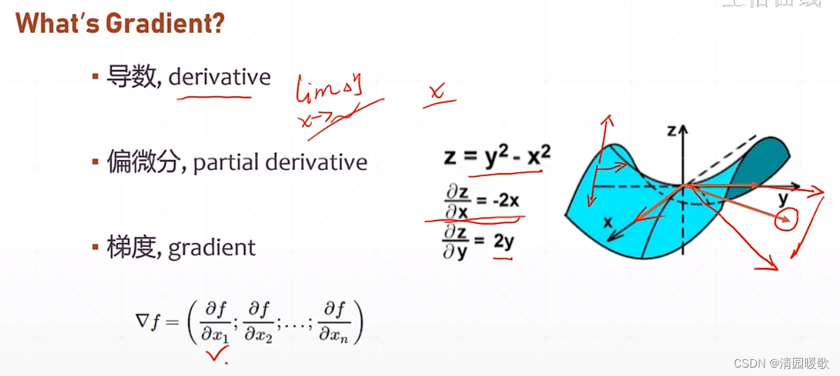
梯度就是所有偏微分一起综合考虑
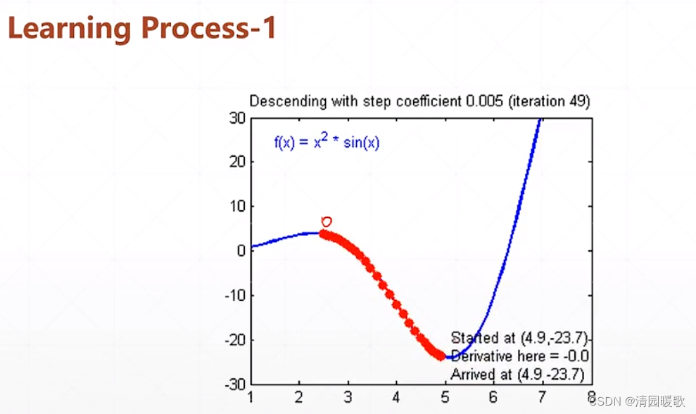
如下图感受梯度,梯度方向代表函数值增大的方向,梯度的模(长度)代表函数增大的速度(速率)
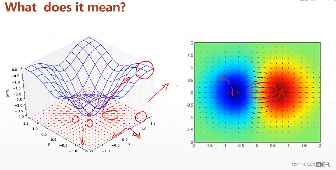
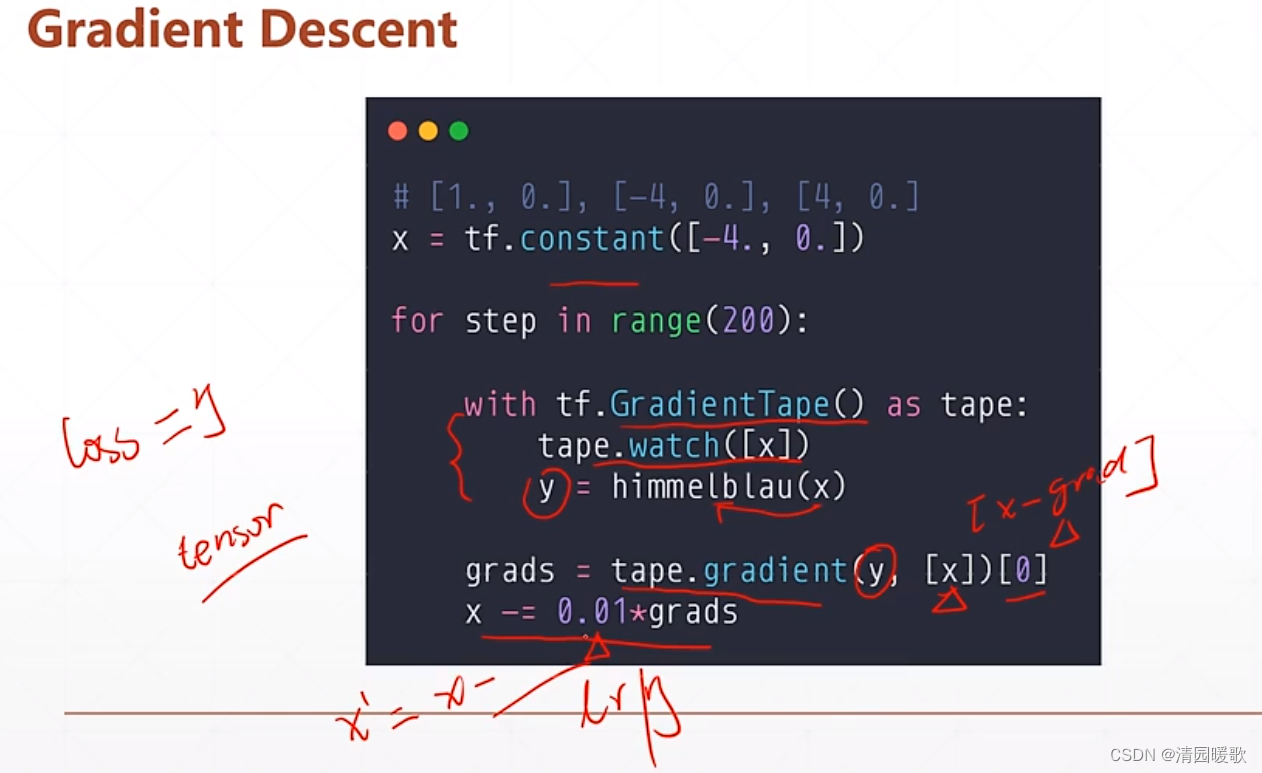
那么梯度如何帮助我们搜索 loss 的最小值呢?
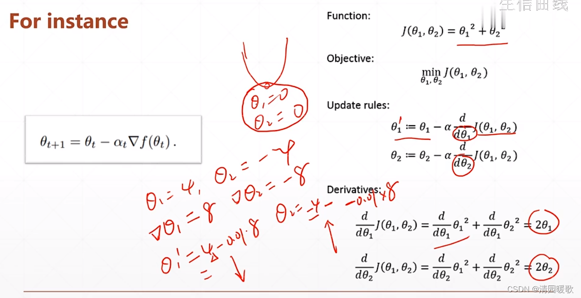
也就是把当前的参数值,沿梯度相反的方向行进更新

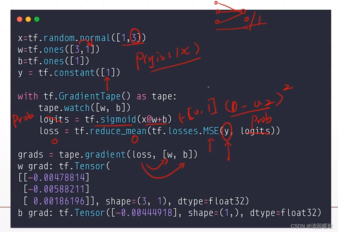
来看一个实例:

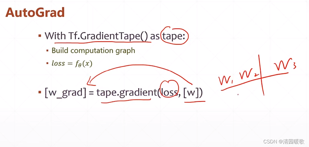
y 的输出out 是None,因为 y=x*w 没有被包在 tf.GradientTape()

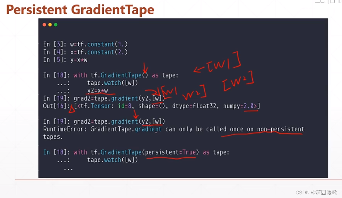
但上述的方法只能求解一次,求解完就会自动释放掉相关的资源
如果要调用两次的话,就需要调用 persistent 的功能
二阶求导:

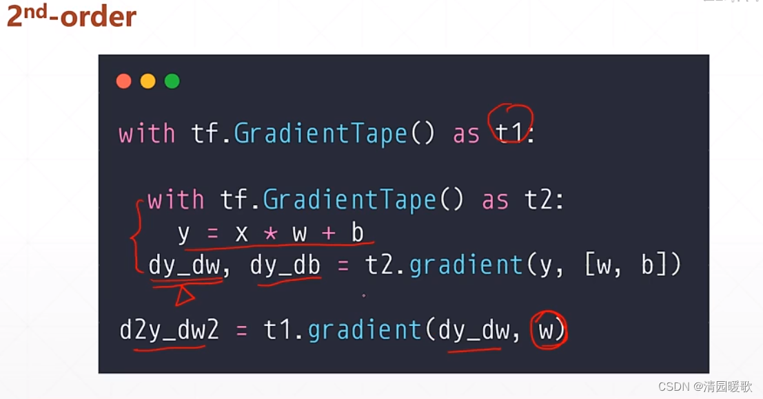
代码:chapter03:TF02-2nd_derivative.py
二、激活函数及其梯度
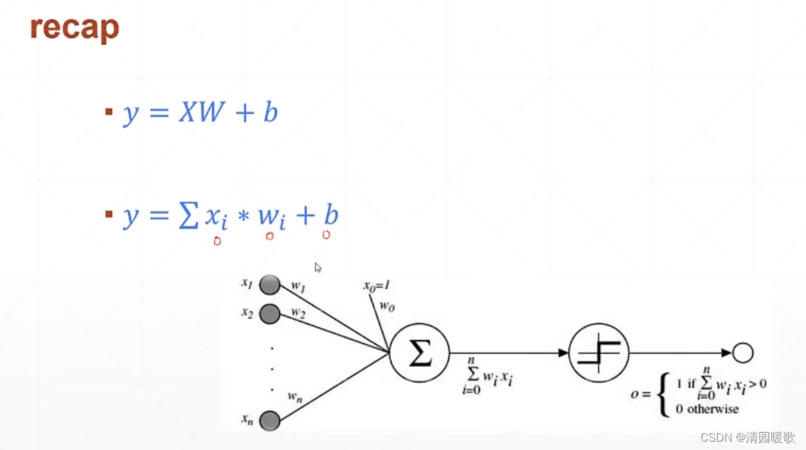
2.1 最简单的阶梯激活函数
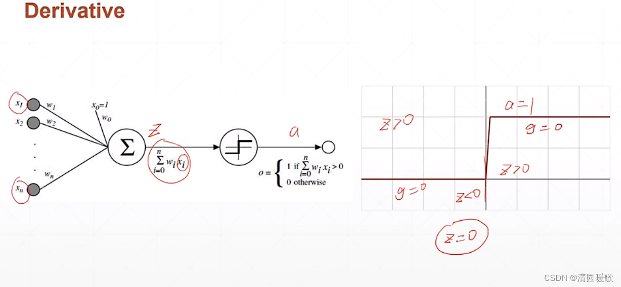
由上图可知,这个z变量必须>0,才会激活,不然就处于一个睡眠状态,不会输出一个电平值,这就是 激活函数 激活 的来源
但这个激活函数存在一个最终的概念,就是不可导的,不能直接使用梯度下降的方法进行优化,在当时使用了一个启发式搜索的方法来求解这样一个单层感知器的最优解的情况
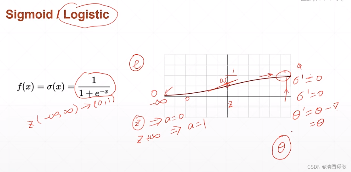
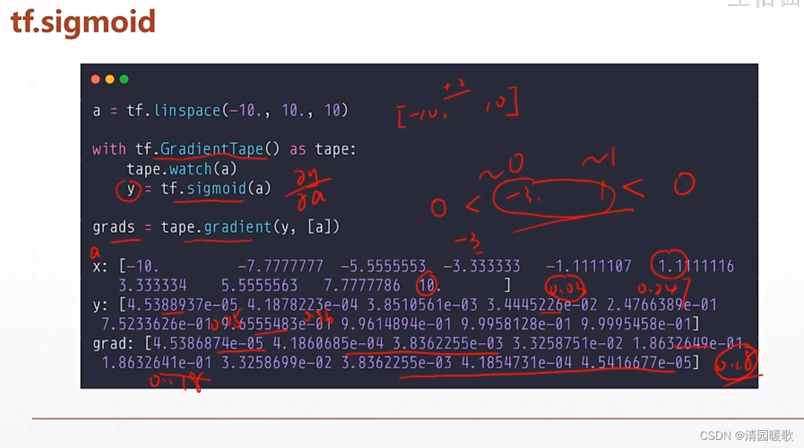
2.2 sigmoid / logistic(tf.sigmoid)
为了解决单层感知器的激活函数,激活阶梯函数不可导的情况,科学家提出了一个连续光滑的函数,就是 sigmoid / logistic


但是到正无穷和负无穷时,导数接近于0,此时 θ 长时间得不到更新,就出现了 梯度离散 现象
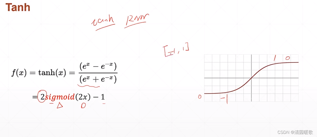
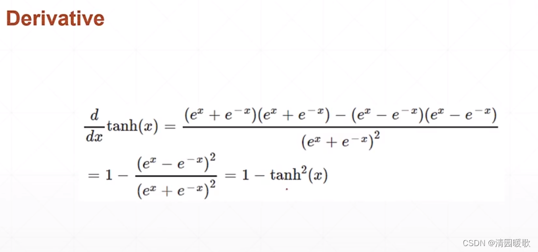
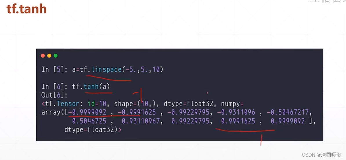
2.3 tanh(tf.tanh)
在 RNN 中用的比较多
可以由 sigmoid 转化来,x轴平面压缩 1/2 即 2x,y轴放大2倍即(0, 2),再减1
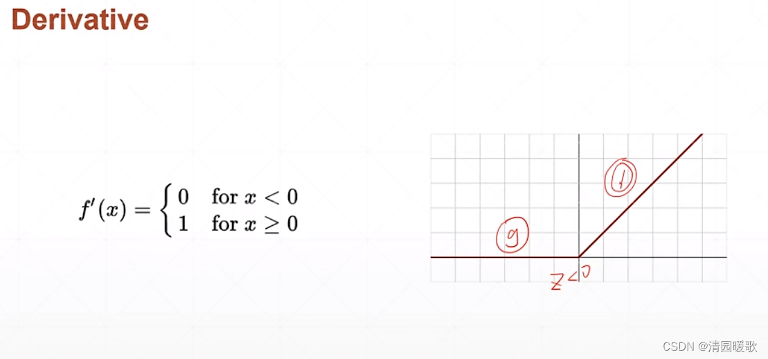
2.4 ReLU(tf.nn.relu)
全名:整型的线性单元 Rectified Linear Unit

小于0时梯度为0,大于0时梯度为1,所以向后传播时梯度计算起来非常方便,不会放大也不会缩小,保持梯度不变,很大程度上减少了出现梯度离散和梯度爆炸的情况
leaky_relu 是小于0的返回一个 kx,k很小;大于0时就是 k=1

三、损失函数及其梯度

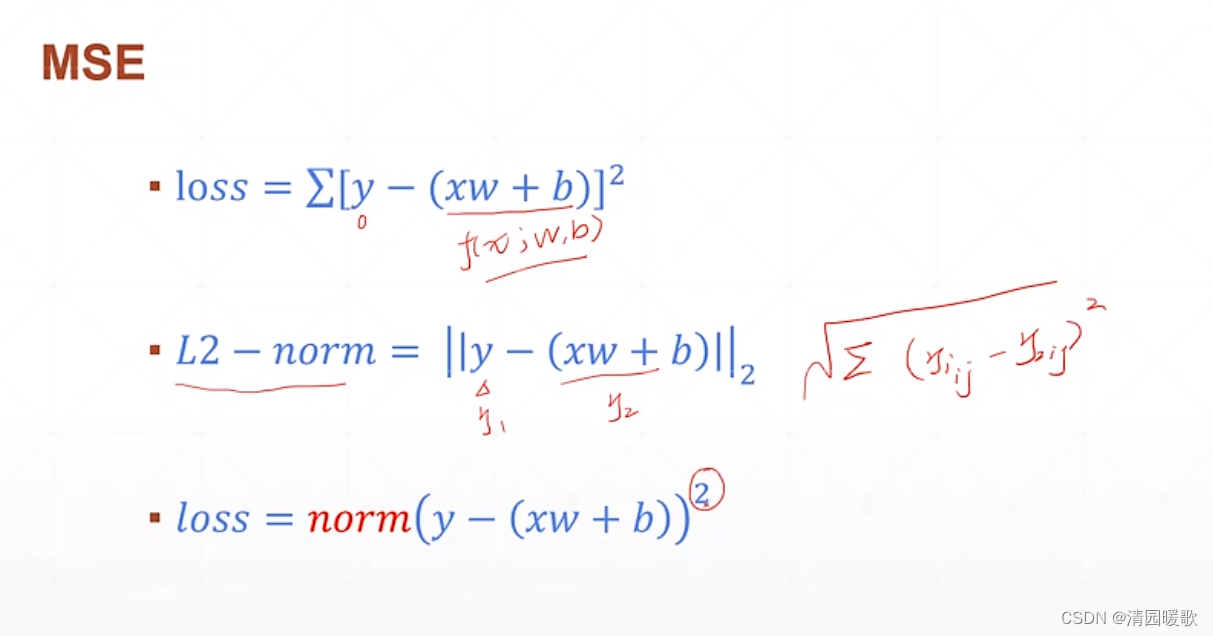
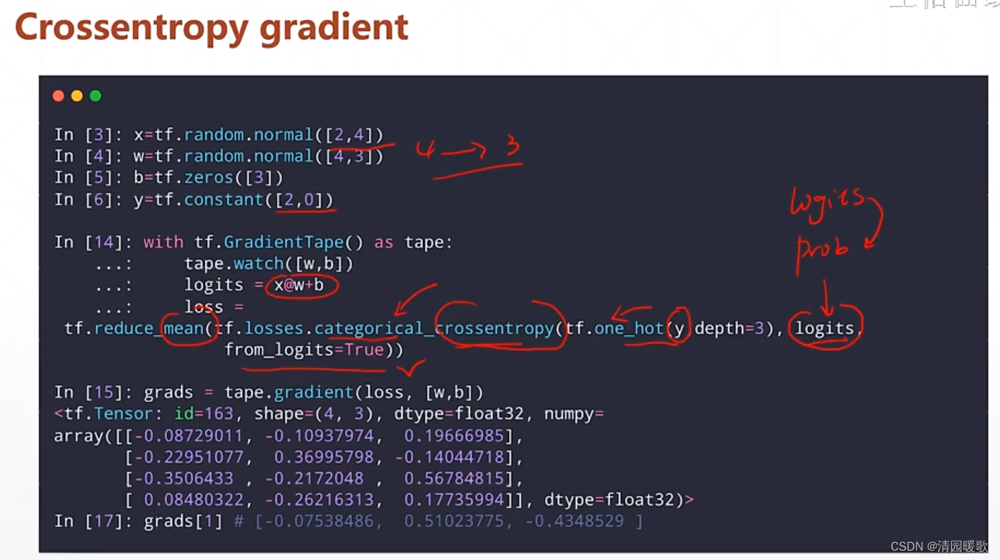
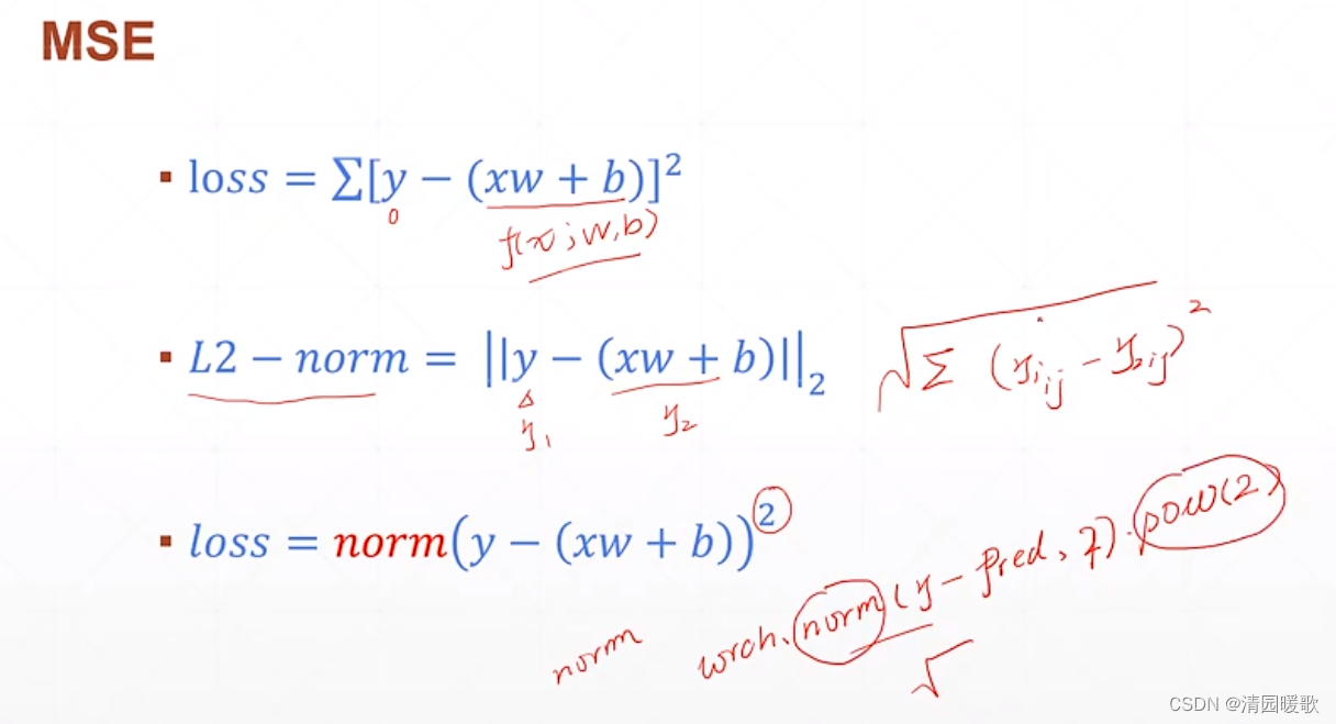 梯度:
梯度:
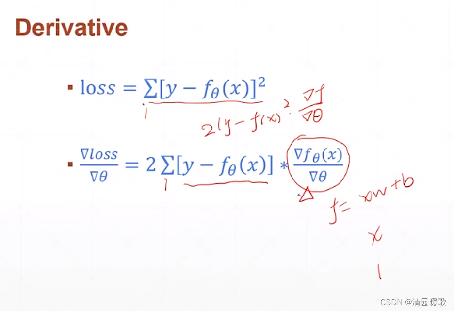

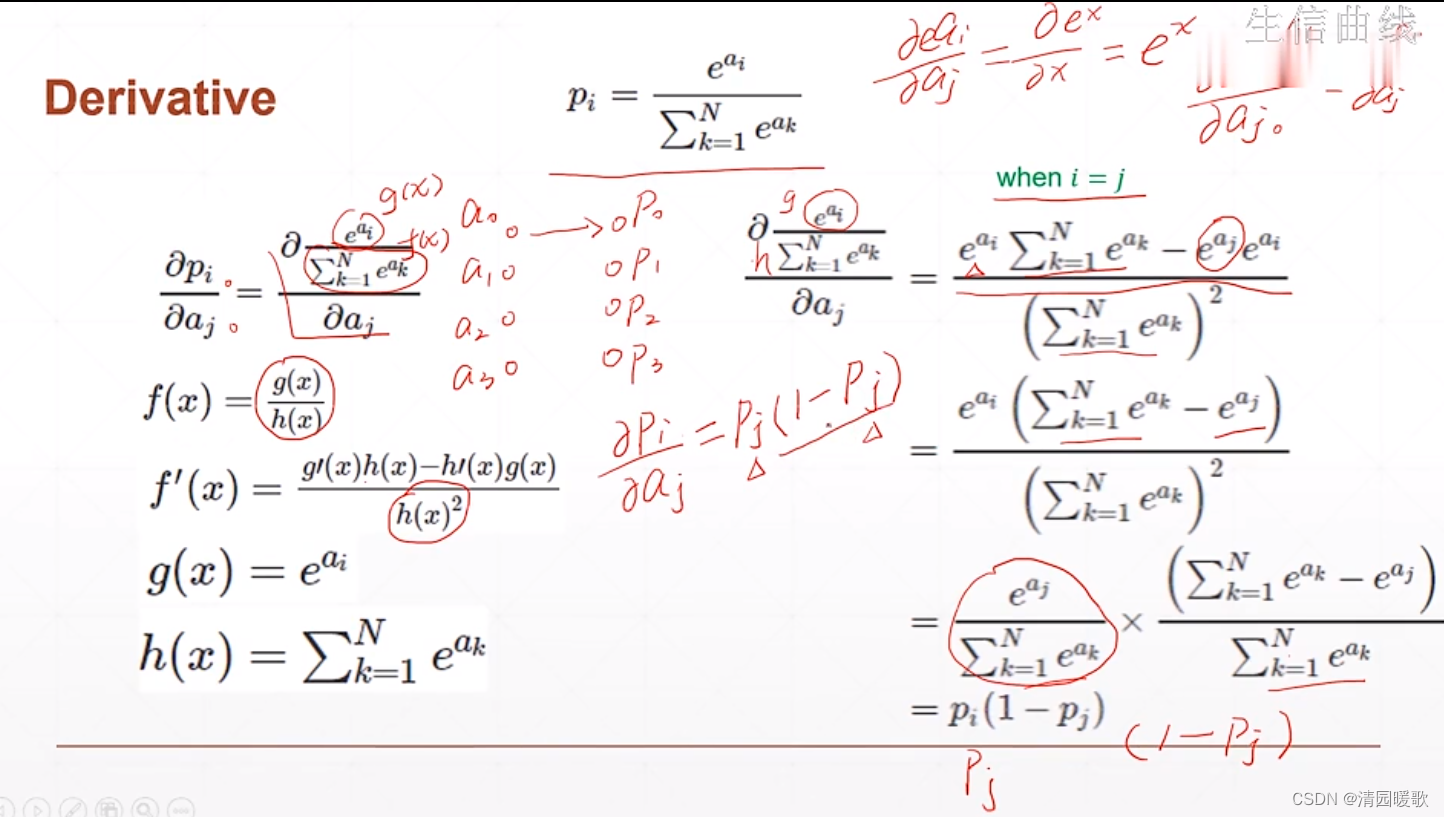
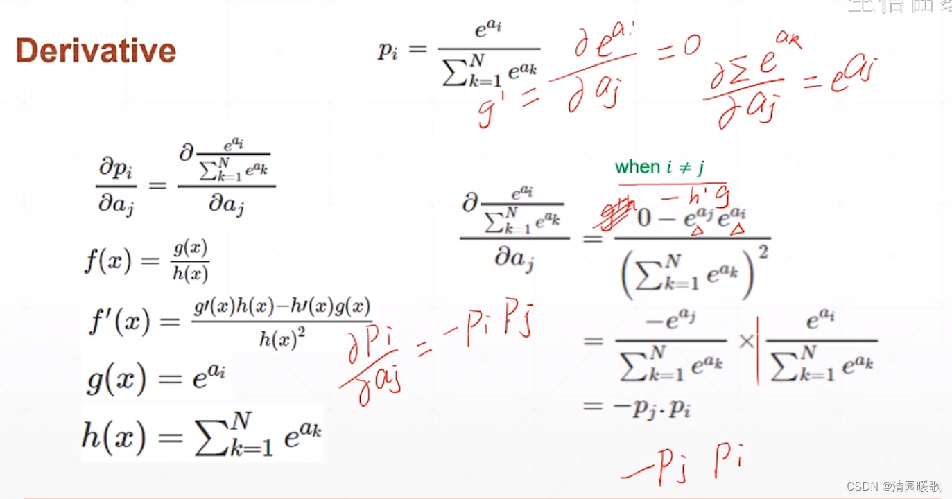
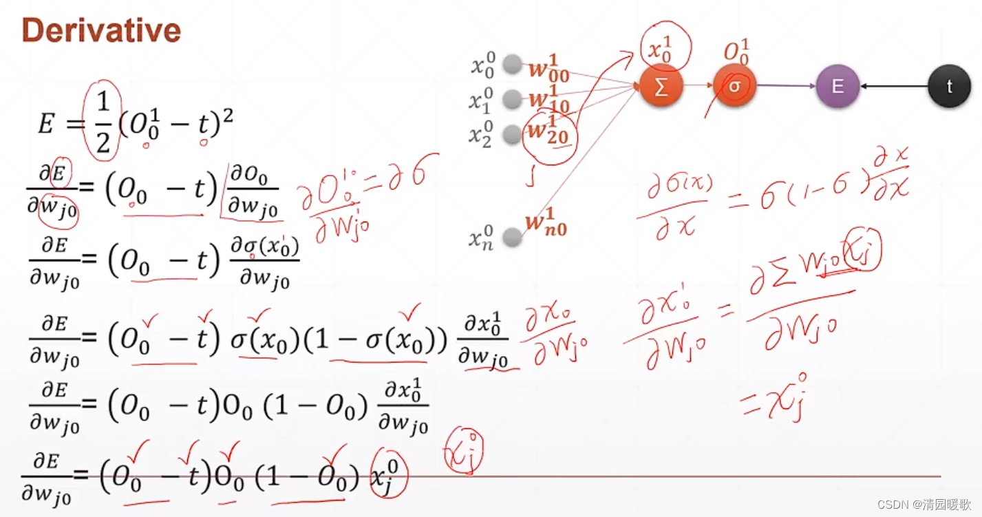
 求导:
求导:

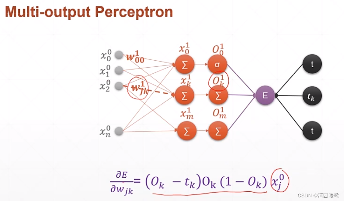
四、单、多输出感知机梯度
4.1 单层感知机
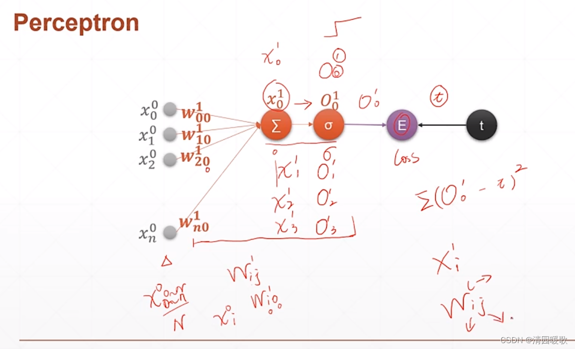

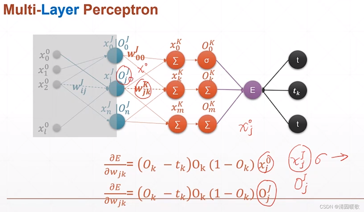
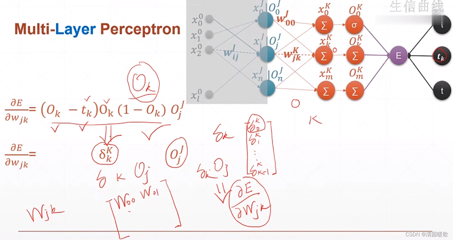
4.2 多层感知机
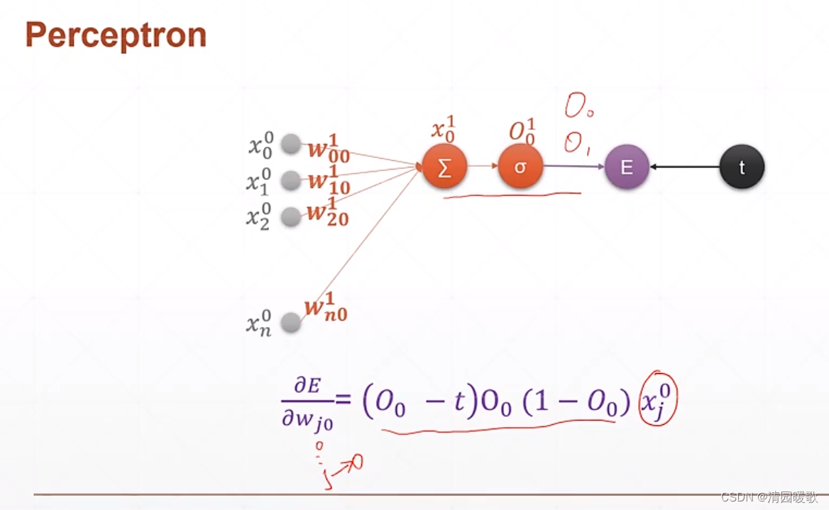
 要求的就是 E(loss)对 wjk的导数


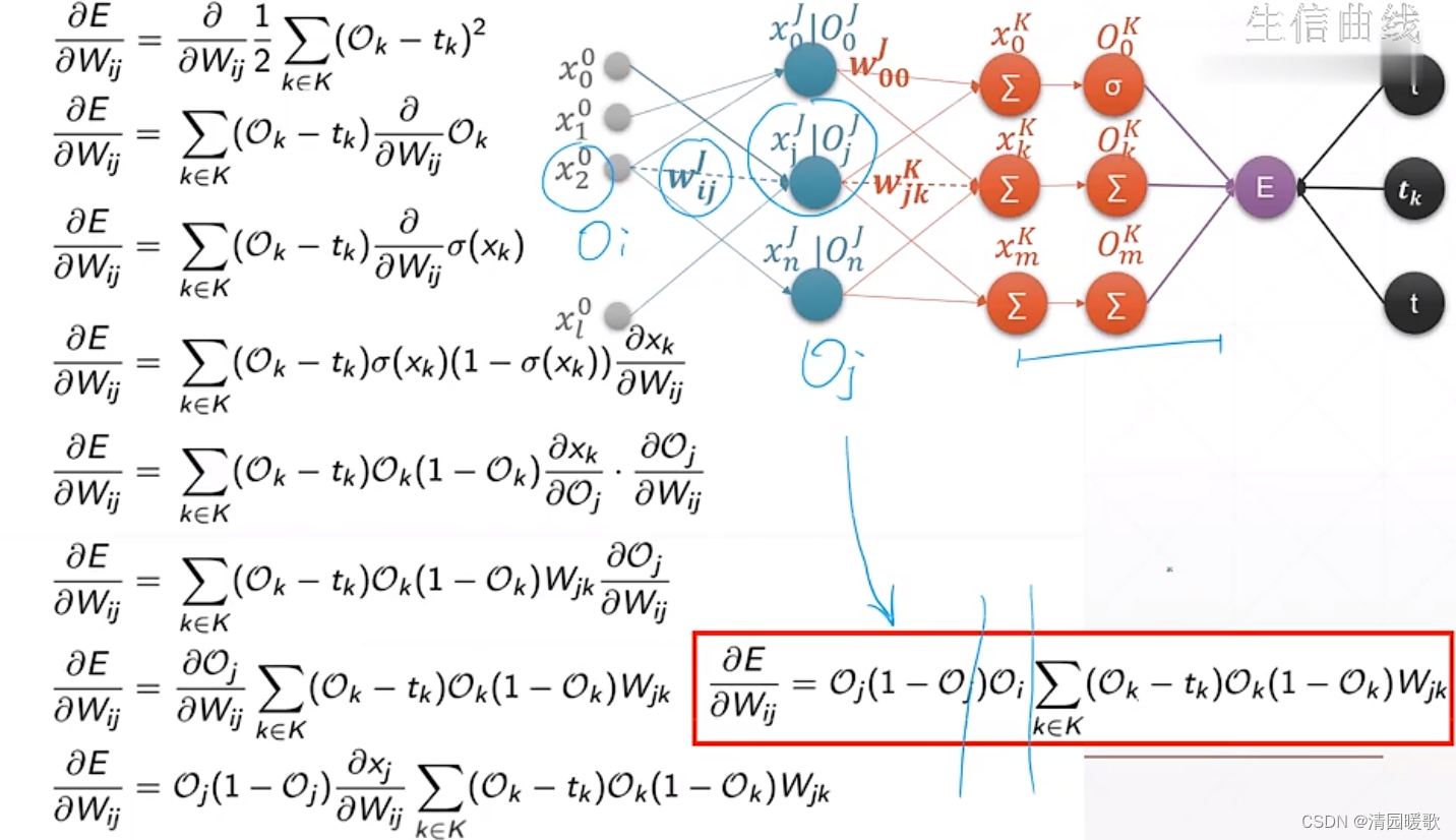
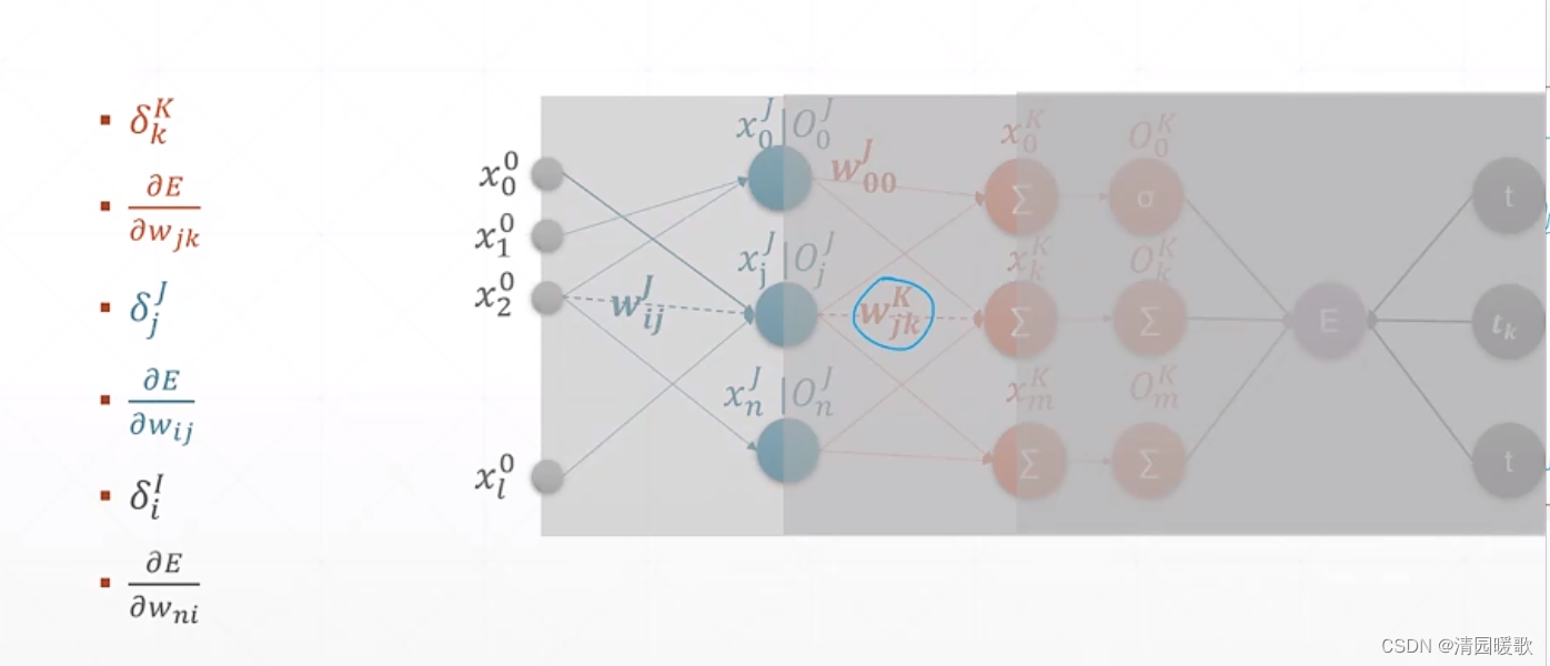
4.3 链式法则


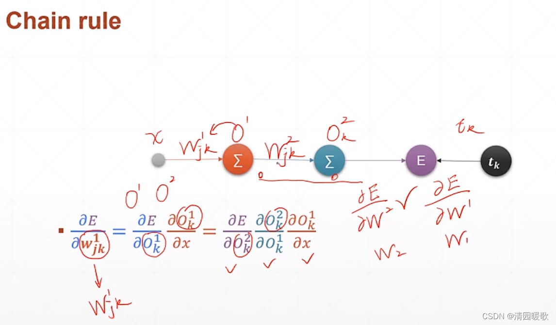
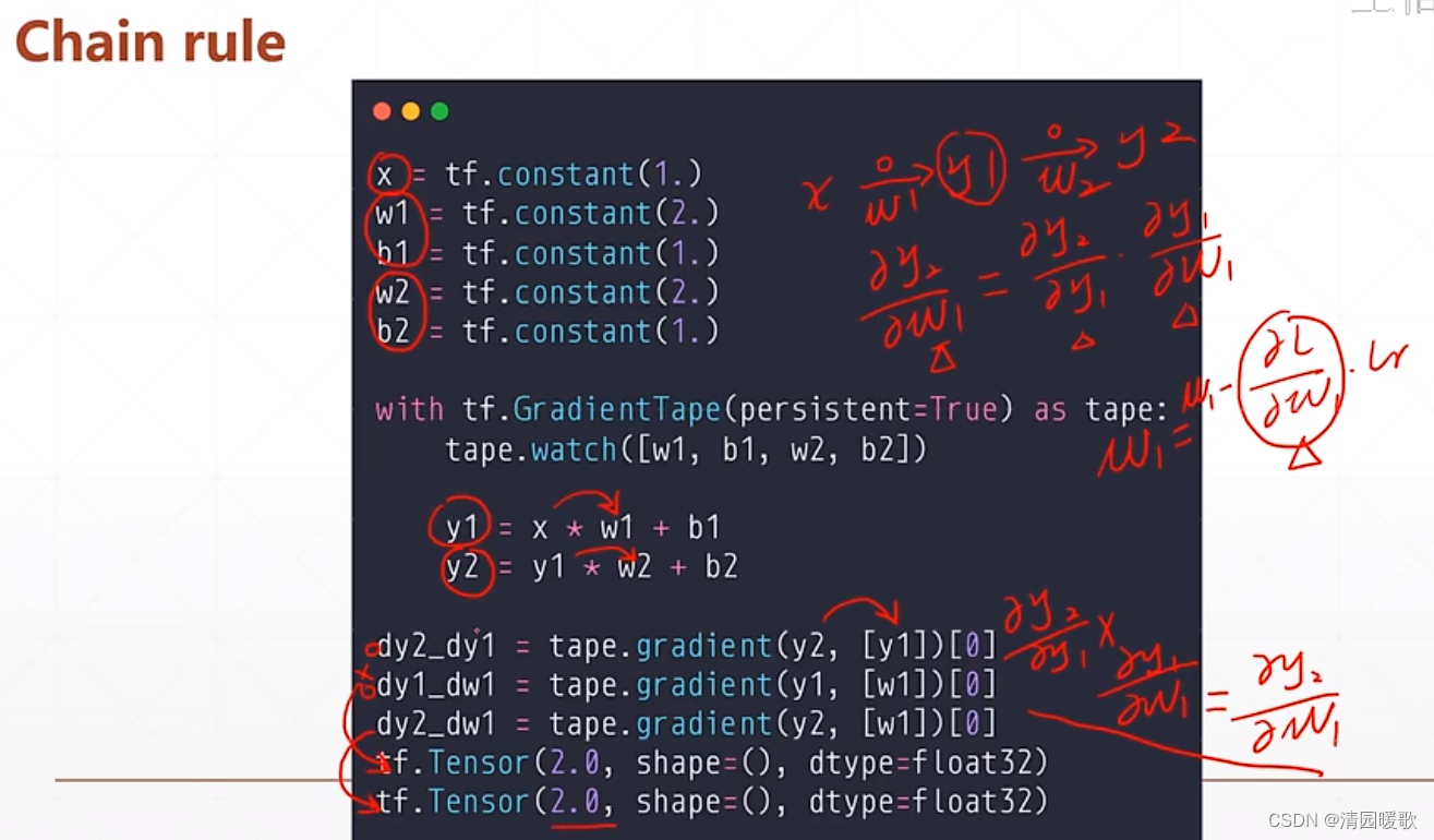
4.4 多层感知机梯度


4.5 Himmelblau函数优化
该函数是一个二维的形式,有四个角,最低点都是0

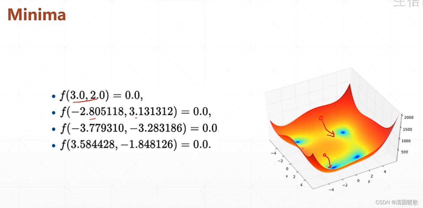

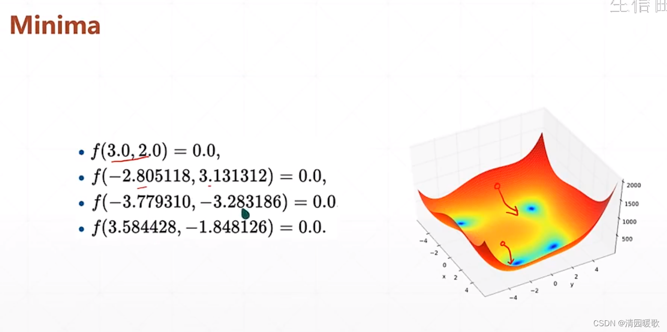
 改变初始点,会找到4个不同的最低点
4.6 FashionMNIST实战
代码:
import tensorflow as tf
from tensorflow import keras
from tensorflow.keras import datasets, layers, optimizers, Sequential, metrics


# 预处理函数
def preprocess(x, y):

    x = tf.cast(x, dtype=tf.float32) / 255.
    y = tf.cast(y, dtype=tf.int32)

    return x, y

(x, y), (x_test, y_test) = datasets.fashion_mnist.load_data()
#print(y[0]) # 9
print(x.shape, y.shape)

batchsz = 128
db = tf.data.Dataset.from_tensor_slices((x, y)) # 构造数据集
# 它可以将一个 Tensor 切片成多个 Tensor,并将其作为数据集返回。
# 可以使用该函数对数据进行预处理,然后使用 TensorFlow 的数据集 API 进行操作。
db = db.map(preprocess).shuffle(10000).batch(batchsz)

db_test = tf.data.Dataset.from_tensor_slices((x_test, y_test)) # 构造数据集
db_test = db_test.map(preprocess).batch(batchsz)

db_iter = iter(db)
sample = next(db_iter)
print('batch:', sample[0].shape, sample[1].shape)

model = Sequential([
    layers.Dense(256, activation=tf.nn.relu), # [b, 784] => [b, 256]
    layers.Dense(128, activation=tf.nn.relu), # [b, 256] => [b, 128]
    layers.Dense(64, activation=tf.nn.relu),  # [b, 128] => [b, 64]
    layers.Dense(32, activation=tf.nn.relu),  # [b, 64] => [b, 32]
    layers.Dense(10)   # [b, 32] => [b, 10], 330 = 32*10 + 10
])
model.build(input_shape=[None, 28*28])
model.summary()
# 给个优化器, w = w - lr * grad
optimizer = optimizers.Adam(lr=1e-3)

def main():

    # 完成数据的前向传播
    for epoch in range(30):

        for step, (x, y) in enumerate(db): # 60000 / 128 = 468.75

            # x: [b, 28, 28]
            # y: [b]
            x = tf.reshape(x, [-1, 28*28])

            with tf.GradientTape() as tape:
                # [b, 784] => [b, 10]
                logits = model(x)
                y_onehot = tf.one_hot(y, depth=10)
                # b
                loss_mse = tf.reduce_mean(tf.losses.MSE(y_onehot, logits))
                loss_ce = tf.losses.categorical_crossentropy(y_onehot, logits, from_logits=True)
                loss_ce = tf.reduce_mean(loss_ce)
                # 如果输入给 bce 的是一个 logit 值(值域范围 [-∞, +∞] ),则应该设置 from_logits=True
                # 如果输入给 bce 的是一个概率值 probability (值域范围 [0, 1] ),则应该设置为 from_logits=False

            grads = tape.gradient(loss_ce, model.trainable_variables) # 计算梯度
                                                            # model.trainable_variables返回所有可训练参数
            optimizer.apply_gradients(zip(grads, model.trainable_variables)) # zip是把两个变量相同标号的拼到一起
                                                            # 梯度在前,参数在后
            if step % 100 == 0:
                print(epoch, step, 'loss:', float(loss_ce), float(loss_mse))

        # test
        total_correct = 0
        total_num = 0
        for x, y in db_test:
            # x: [b, 28, 28]
            # y: [b]
            x = tf.reshape(x, [-1, 28 * 28])
            # [b, 10]
            logits = model(x)
            # logits => prob, [b, 10]
            prob = tf.nn.softmax(logits, axis=1)
            # [b, 10] => [b], int64
            pred = tf.argmax(prob, axis=1)
            pred = tf.cast(pred, dtype=tf.int32)
            # pred: [b]
            # y: [b]
            # correct: [b], True: equal, False: not equal
            correct = tf.equal(pred, y)
            correct = tf.reduce_sum(tf.cast(correct, dtype=tf.int32)) # 这里的 correct 是一个 Tensor

            total_correct += int(correct) # 每个 for 的相加
            total_num += x.shape[0]

        acc = total_correct / total_num
        print(epoch, 'test acc:', acc)

# 这里用的是 loss_ce 的 loss,也可以试试 loss_mse 的 loss
# 两个好处:
# (1)有5层,比2、3层多了很多参数
# (2)用了 adam 的优化器
# 最后 acc 在 0.892,fashionmnist 比 mnist 要复杂

if __name__ == '__main__':
    main()
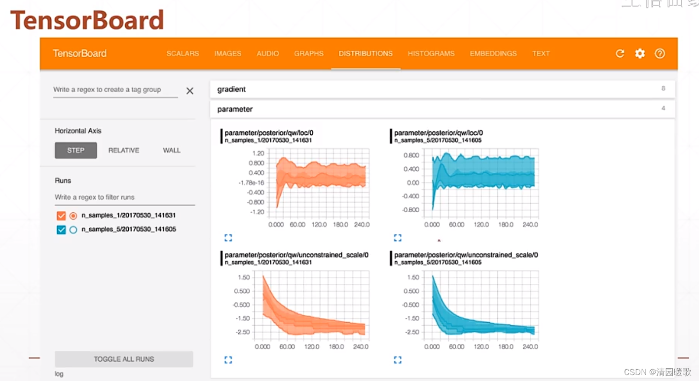
4.7 TensorBoard可视化
想要查看过程中任意部分,直接 print 的话,如果是 deep net 那么会有很多参数和图片,很难看出过程部分

在 tensorlfow 中这个监视工具叫 TensorBoard
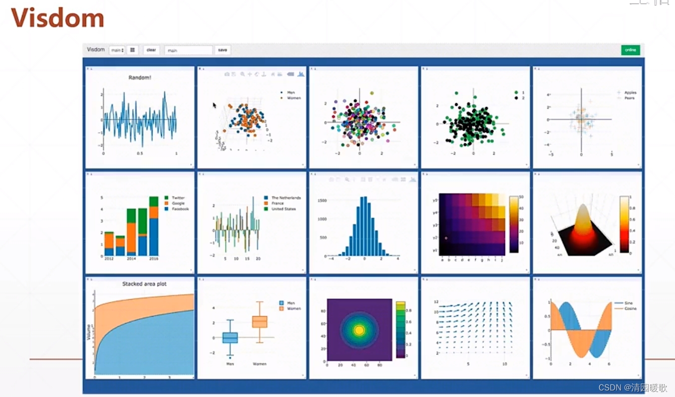
在 pytorch 中,叫 Visdom
但这两个并不局限使用,可以互相用

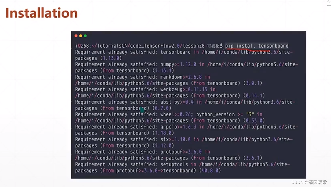
4.7.1 Installation
新版 tensorflow 好像会自动安装,没有直接 pip 安装
 工作原理:cpu 会运行程序给磁盘的某个目录写程序,里面就会更新包含数据如loss,讲目录告诉监听器listen,监听器就会监听这个目录,这样打开web网页,listen有数据就会传到web显示
4.7.2 Curves
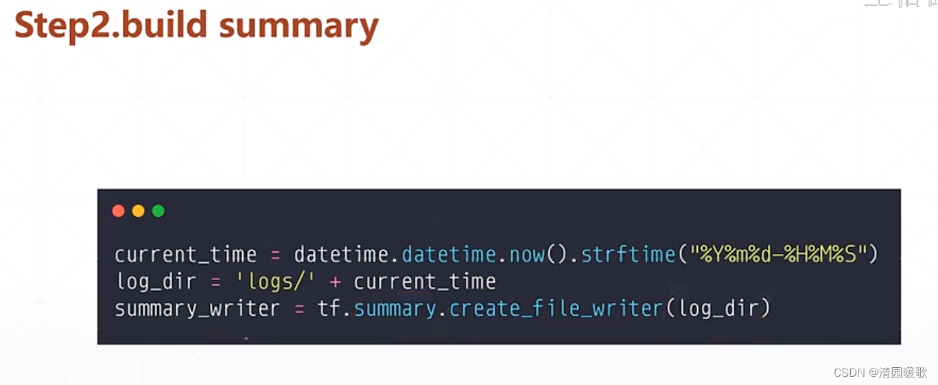
(1)新建目录(2)建立日志(3)数据喂给这个日志summary

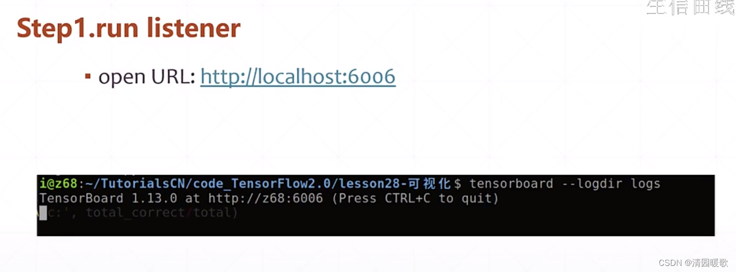
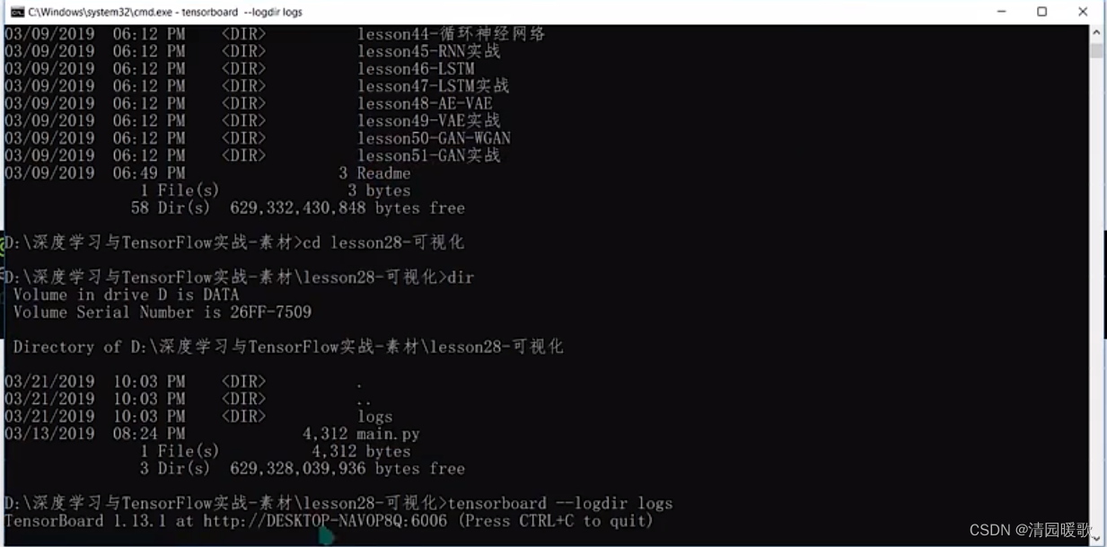
进入命令行cmd:

进入监听目录,然后输入
tensorboard --logdir logs
就可以在 6006 端口查看,给的地址不对的话,就进入 localhost:6006
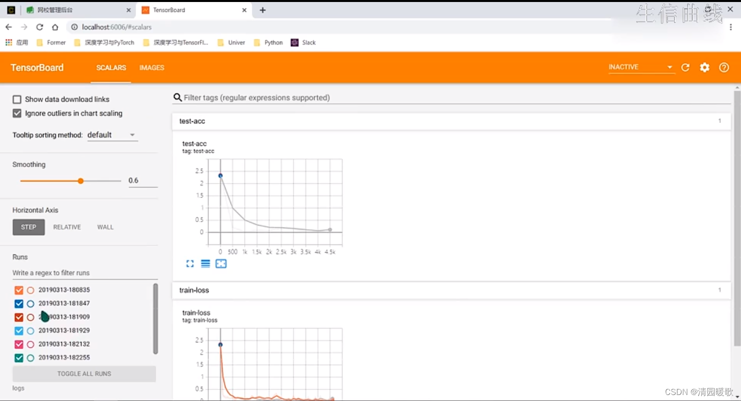
4.7.3 Image Visualization
step就是横轴,loss那里就是纵轴,'loss'就是名称
喂一个标量的数据:
 喂一个图片的数据:


喂多张图片:
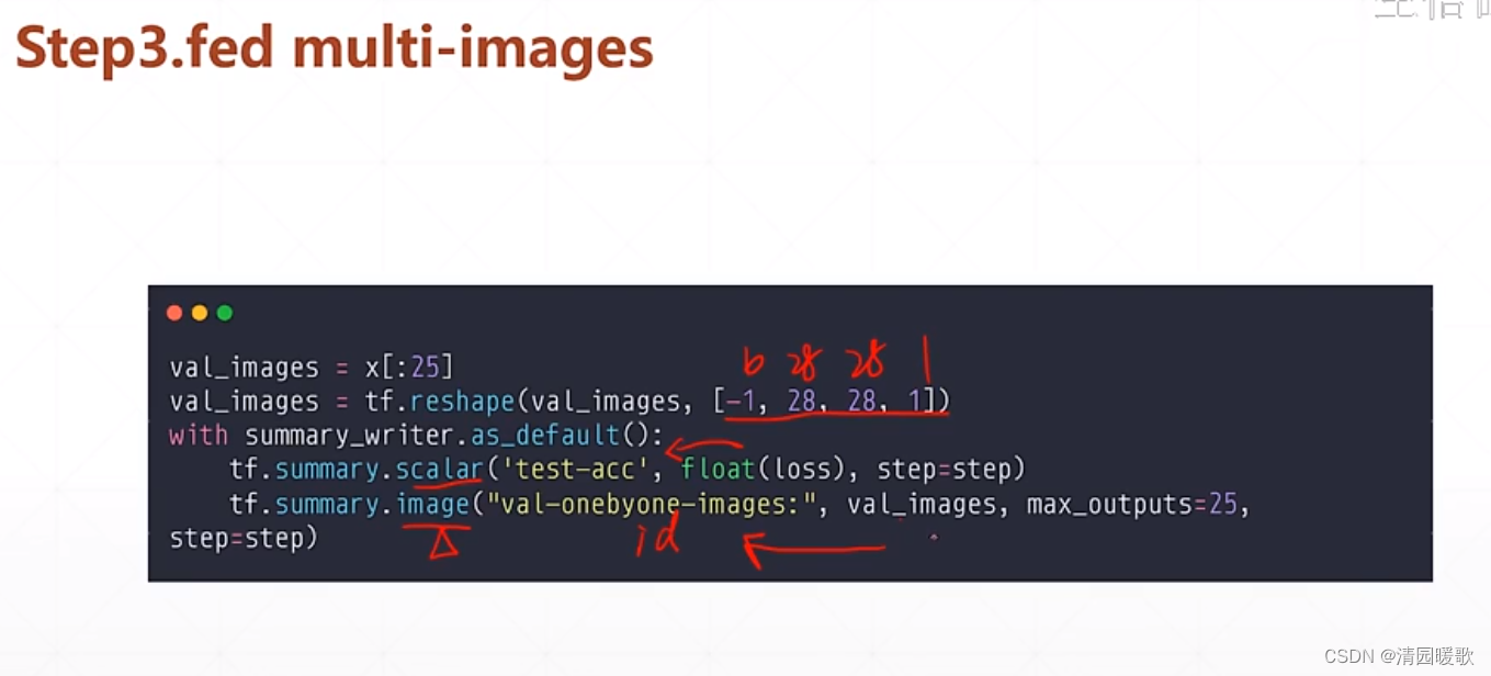
 但是这样没有组合起来显示,是一个一个显示的,浪费了大量的资源
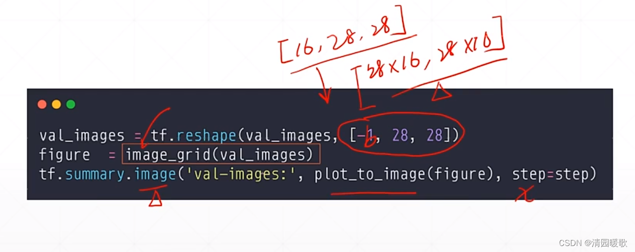
要想组合起来,tensorflow没有提供这个工具,需要我们自己写一个函数,这里是 image_grid

chapter03 - TF06
代码:
# 可视化
# 打开ip地址:localhost:6006
import os

os.environ['TF_CPP_MIN_LOG_LEVEL'] = '2'

import tensorflow as tf
from tensorflow.keras import datasets, layers, optimizers, Sequential, metrics
import datetime
from matplotlib import pyplot as plt
import io

assert tf.__version__.startswith('2.')


def preprocess(x, y):
    x = tf.cast(x, dtype=tf.float32) / 255.
    y = tf.cast(y, dtype=tf.int32)

    return x, y


def plot_to_image(figure):
    """Converts the matplotlib plot specified by 'figure' to a PNG image and
    returns it. The supplied figure is closed and inaccessible after this call."""
    # Save the plot to a PNG in memory.
    buf = io.BytesIO()
    plt.savefig(buf, format='png')
    # Closing the figure prevents it from being displayed directly inside
    # the notebook.
    plt.close(figure)
    buf.seek(0)
    # Convert PNG buffer to TF image
    image = tf.image.decode_png(buf.getvalue(), channels=4)
    # Add the batch dimension
    image = tf.expand_dims(image, 0)
    return image


def image_grid(images):
    """Return a 5x5 grid of the MNIST images as a matplotlib figure."""
    # Create a figure to contain the plot.
    figure = plt.figure(figsize=(10, 10))
    for i in range(25):
        # Start next subplot.
        plt.subplot(5, 5, i + 1, title='name')
        plt.xticks([])
        plt.yticks([])
        plt.grid(False)
        plt.imshow(images[i], cmap=plt.cm.binary)

    return figure


batchsz = 128
(x, y), (x_val, y_val) = datasets.mnist.load_data()
print('datasets:', x.shape, y.shape, x.min(), x.max())

db = tf.data.Dataset.from_tensor_slices((x, y))
db = db.map(preprocess).shuffle(60000).batch(batchsz).repeat(10)

ds_val = tf.data.Dataset.from_tensor_slices((x_val, y_val))
ds_val = ds_val.map(preprocess).batch(batchsz, drop_remainder=True)

network = Sequential([layers.Dense(256, activation='relu'),
                      layers.Dense(128, activation='relu'),
                      layers.Dense(64, activation='relu'),
                      layers.Dense(32, activation='relu'),
                      layers.Dense(10)])
network.build(input_shape=(None, 28 * 28))
network.summary()

optimizer = optimizers.Adam(lr=0.01)

current_time = datetime.datetime.now().strftime("%Y%m%d-%H%M%S")
log_dir = 'logs/' + current_time
summary_writer = tf.summary.create_file_writer(log_dir)

# get x from (x,y)
sample_img = next(iter(db))[0]
# get first image instance
sample_img = sample_img[0]
sample_img = tf.reshape(sample_img, [1, 28, 28, 1])
with summary_writer.as_default():
    tf.summary.image("Training sample:", sample_img, step=0)

for step, (x, y) in enumerate(db):

    with tf.GradientTape() as tape:
        # [b, 28, 28] => [b, 784]
        x = tf.reshape(x, (-1, 28 * 28))
        # [b, 784] => [b, 10]
        out = network(x)
        # [b] => [b, 10]
        y_onehot = tf.one_hot(y, depth=10)
        # [b]
        loss = tf.reduce_mean(tf.losses.categorical_crossentropy(y_onehot, out, from_logits=True))

    grads = tape.gradient(loss, network.trainable_variables)
    optimizer.apply_gradients(zip(grads, network.trainable_variables))

    if step % 100 == 0:
        print(step, 'loss:', float(loss))
        with summary_writer.as_default():
            tf.summary.scalar('train-loss', float(loss), step=step)

            # evaluate
    if step % 500 == 0:
        total, total_correct = 0., 0

        for _, (x, y) in enumerate(ds_val):
            # [b, 28, 28] => [b, 784]
            x = tf.reshape(x, (-1, 28 * 28))
            # [b, 784] => [b, 10]
            out = network(x)
            # [b, 10] => [b]
            pred = tf.argmax(out, axis=1)
            pred = tf.cast(pred, dtype=tf.int32)
            # bool type
            correct = tf.equal(pred, y)
            # bool tensor => int tensor => numpy
            total_correct += tf.reduce_sum(tf.cast(correct, dtype=tf.int32)).numpy()
            total += x.shape[0]

        print(step, 'Evaluate Acc:', total_correct / total)

        # print(x.shape)
        val_images = x[:25]
        val_images = tf.reshape(val_images, [-1, 28, 28, 1])
        with summary_writer.as_default():
            tf.summary.scalar('test-acc', float(total_correct / total), step=step)
            tf.summary.image("val-onebyone-images:", val_images, max_outputs=25, step=step)

            val_images = tf.reshape(val_images, [-1, 28, 28])
            figure = image_grid(val_images)
            tf.summary.image('val-images:', plot_to_image(figure), step=step)