分类预测 | MATLAB实现WOA-CNN-BiGRU鲸鱼算法优化卷积双向门控循环单元数据分类预测
分类效果


基本描述
1.Matlab实现WOA-CNN-BiGRU多特征分类预测,多特征输入模型,运行环境Matlab2020b及以上;
2.基于鲸鱼算法(WOA)优化卷积神经网络-双向门控循环单元(CNN-BiGRU)分类预测,优化参数为,学习率,隐含层节点,正则化参数;
3.多特征输入单输出的二分类及多分类模型。程序内注释详细,直接替换数据就可以用;
程序语言为matlab,程序可出分类效果图,迭代优化图,混淆矩阵图;
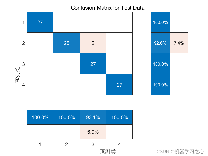
4.data为数据集,输入12个特征,分四类;运行主程序即可,其余为函数文件,无需运行,可在下载区获取数据和程序内容。
模型描述
CNN 是一种前馈型神经网络,广泛应用于深度学习领域,主要由卷积层、池化层和全连接层组成,输入特征向量可以为多维向量组,采用局部感知和权值共享的方式。卷积层对原始数据提取特征量,深度挖掘数据的内在联系,池化层能够降低网络复杂度、减少训练参数,全连接层将处理后的数据进行合并,计算分类和回归结果。
BiGRU是LSTM的一种改进模型,将遗忘门和输入门集成为单一的更新门,同时混合了神经元状态和隐藏状态,可有效地缓解循环神经网络中“梯度消失”的问题,并能够在保持训练效果的同时减少训练参数。
程序设计
- 完整程序和数据获取方式私信博主回复MATLAB实现WOA-CNN-BiGRU鲸鱼算法优化卷积双向门控循环单元数据分类预测。
% The Whale Optimization Algorithm
function [Best_Cost,Best_pos,curve]=WOA(pop,Max_iter,lb,ub,dim,fobj)

% initialize position vector and score for the leader
Best_pos=zeros(1,dim);
Best_Cost=inf; %change this to -inf for maximization problems


%Initialize the positions of search agents
Positions=initialization(pop,dim,ub,lb);

curve=zeros(1,Max_iter);

t=0;% Loop counter

% Main loop
while t<Max_iter
    for i=1:size(Positions,1)

        % Return back the search agents that go beyond the boundaries of the search space
        Flag4ub=Positions(i,:)>ub;
        Flag4lb=Positions(i,:)<lb;
        Positions(i,:)=(Positions(i,:).*(~(Flag4ub+Flag4lb)))+ub.*Flag4ub+lb.*Flag4lb;

        % Calculate objective function for each search agent
        fitness=fobj(Positions(i,:));

        % Update the leader
        if fitness<Best_Cost % Change this to > for maximization problem
            Best_Cost=fitness; % Update alpha
            Best_pos=Positions(i,:);
        end

    end

    a=2-t*((2)/Max_iter); % a decreases linearly fron 2 to 0 in Eq. (2.3)

    % a2 linearly dicreases from -1 to -2 to calculate t in Eq. (3.12)
    a2=-1+t*((-1)/Max_iter);

    % Update the Position of search agents
    for i=1:size(Positions,1)
        r1=rand(); % r1 is a random number in [0,1]
        r2=rand(); % r2 is a random number in [0,1]

        A=2*a*r1-a;  % Eq. (2.3) in the paper
        C=2*r2;      % Eq. (2.4) in the paper


        b=1;               %  parameters in Eq. (2.5)
        l=(a2-1)*rand+1;   %  parameters in Eq. (2.5)

        p = rand();        % p in Eq. (2.6)

        for j=1:size(Positions,2)

            if p<0.5
                if abs(A)>=1
                    rand_leader_index = floor(pop*rand()+1);
                    X_rand = Positions(rand_leader_index, :);
                    D_X_rand=abs(C*X_rand(j)-Positions(i,j)); % Eq. (2.7)
                    Positions(i,j)=X_rand(j)-A*D_X_rand;      % Eq. (2.8)

                elseif abs(A)<1
                    D_Leader=abs(C*Best_pos(j)-Positions(i,j)); % Eq. (2.1)
                    Positions(i,j)=Best_pos(j)-A*D_Leader;      % Eq. (2.2)
                end

            elseif p>=0.5

                distance2Leader=abs(Best_pos(j)-Positions(i,j));
                % Eq. (2.5)
                Positions(i,j)=distance2Leader*exp(b.*l).*cos(l.*2*pi)+Best_pos(j);

            end

        end
    end
    t=t+1;
    curve(t)=Best_Cost;
    [t Best_Cost]
end
参考资料
[1] https://blog.csdn.net/kjm13182345320/article/details/129036772?spm=1001.2014.3001.5502
[2] https://blog.csdn.net/kjm13182345320/article/details/128690229