写在前面:博主是一只经过实战开发历练后投身培训事业的“小山猪”,昵称取自动画片《狮子王》中的“彭彭”,总是以乐观、积极的心态对待周边的事物。本人的技术路线从Java全栈工程师一路奔向大数据开发、数据挖掘领域,如今终有小成,愿将昔日所获与大家交流一二,希望对学习路上的你有所助益。同时,博主也想通过此次尝试打造一个完善的技术图书馆,任何与文章技术点有关的异常、错误、注意事项均会在末尾列出,欢迎大家通过各种方式提供素材。
- 对于文章中出现的任何错误请大家批评指出,一定及时修改。
- 有任何想要讨论和学习的问题可联系我:[email protected]。
- 发布文章的风格因专栏而异,均自成体系,不足之处请大家指正。
英特尔oneAPI人工智能黑客松 - 坚果识别实战
本文关键字:英特尔、oneAPI、人工智能、机器视觉
一、活动介绍

最近英特尔和C站官方再次举办了oneAPI的人工智能黑客松活动,也就是使用英特尔的官方套件去解决一些计算机视觉领域的问题,这次支持组队赛,有两个赛道:
- 赛道一:自动驾驶车辆的对象检测
- 赛道二:使用oneAPI人工智能分析工具包实现任何创意
活动主办方提供了源码案例以及公开课视频教程,并且整体的实现流程也描述的十分清楚,可以方便大家快速上手。笔者虽然一直在人工智能领域工作,但是在机器视觉方面还是接触的比较少,但是查看了相关资料后也能在比较短的时间内实现自己的构想,并且感觉自己也get了新技能,不得不由衷点个赞!
二、环境准备
1. 硬件要求
因为是基于英特尔的套件进行机器视觉方面的工作,所以会用到CPU个GPU资源,需要在Intel的机器上进行开发。当然,如果没有合适的机器,也可以使用官方提供的云环境,小编也是尝试了一下,可以免费申请到半年的使用权,并且配置并不低,可以说是十分良心了。
2. 软件环境
如果想要尽快开始,只需要自行安装一些基础的python环境,能够构建官方的案例即可:https://github.com/idz-cn/2023hackathon/tree/main/computer-vision-track
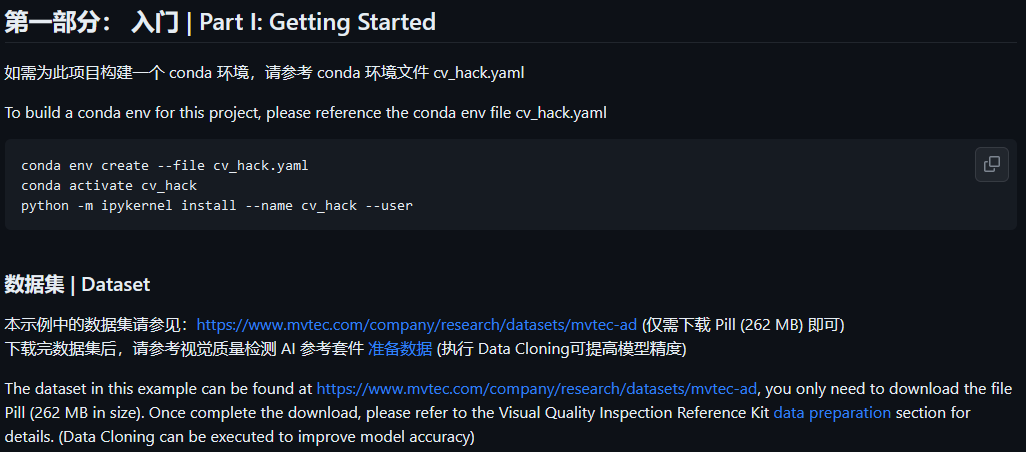
我们可以参考相关的代码,并且可以下载到需要的数据集:https://www.mvtec.com/company/research/datasets/mvtec-ad,里面包含了很多场景的训练图片,可以直接使用。
三、方案实现
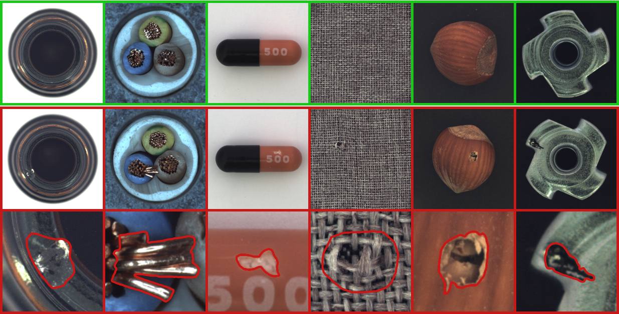
笔者使用的数据集是hazelnut,也就是坚果。我们可以通过训练学习让模型知道什么样的情况是合格的,而什么样的是不合规的。以下将列出部分代码和步骤,详细的可以参考官方案例:
1. 数据集准备
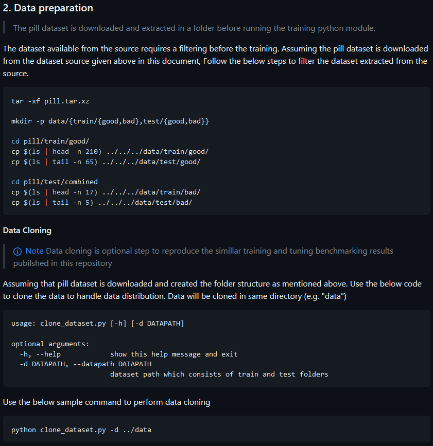
首先要准备好训练集 - train和测试集 - test,并且两者都需要挑选出可以被认可的 - good和不被认可的 - bad,这些图片我们可以从数据集中手动跳转,也可以随机抽取几张,或者参考案例中的数据准备步骤:https://github.com/oneapi-src/visual-quality-inspection#2-data-preparation。
2. 训练和预测
- 对比显示两组图片
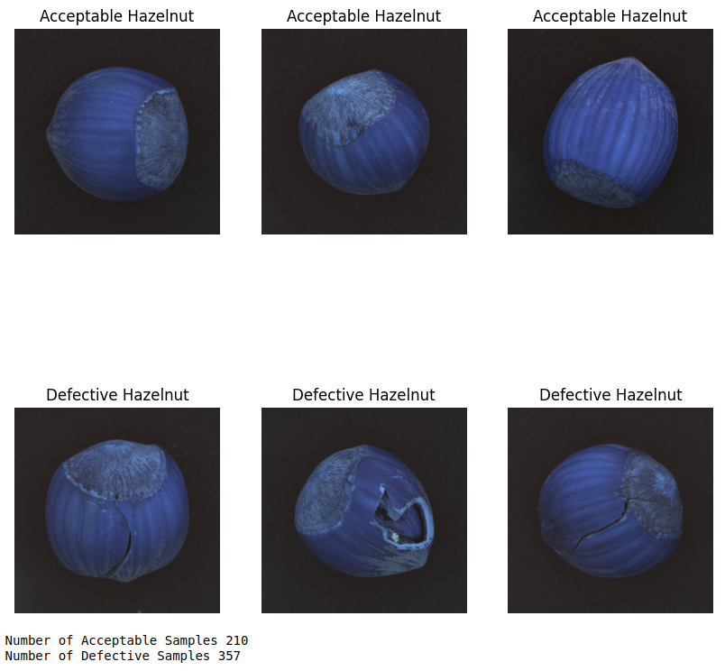
在模型训练阶段,我们先从训练集中抽取一些图片来做对比显示:
import cv2

train_dir = './data/train' # image folder

# get the list of jpegs from sub image class folders
good_imgs = [fn for fn in os.listdir(f'{

      train_dir}/good') if fn.endswith('.png')]
bad_imgs = [fn for fn in os.listdir(f'{

      train_dir}/bad') if fn.endswith('.png')]

# randomly select 3 of each
select_norm = np.random.choice(good_imgs, 3, replace = False)
select_pneu = np.random.choice(bad_imgs, 3, replace = False)

# plotting 2 x 3 image matrix
fig = plt.figure(figsize = (10,10))
for i in range(6):
    if i < 3:
        fp = f'{

      train_dir}/good/{

      select_norm[i]}'
        label = 'Acceptable Cable'
    else:
        fp = f'{

      train_dir}/bad/{

      select_pneu[i-3]}'
        label = 'Defective Cable'
    ax = fig.add_subplot(2, 3, i+1)

    # to plot without rescaling, remove target_size
    fn = cv2.imread(fp)
    fn_gray = cv2.cvtColor(fn, cv2.COLOR_BGR2GRAY)
    plt.imshow(fn, cmap='Greys_r')
    plt.title(label)
    plt.axis('off')
plt.show()
- 接下来需要将图片以数据的形式读取,也就是矩阵或数组的形式
# making n X m matrix
def img2np(path, list_of_filename, size = (64, 64)):
# iterating through each file
for fn in list_of_filename:
fp = path + fn
current_image = cv2.imread(fp)
current_image = cv2.cvtColor(current_image, cv2.COLOR_BGR2GRAY)
# turn that into a vector / 1D array
img_ts = [current_image.ravel()]
try:
# concatenate different images
full_mat = np.concatenate((full_mat, img_ts))
except UnboundLocalError:
# if not assigned yet, assign one
full_mat = img_ts
return full_mat
# run it on our folders
good_images = img2np(f'{
train_dir}/good/', good_imgs)
bad_images = img2np(f'{
train_dir}/bad/', bad_imgs)
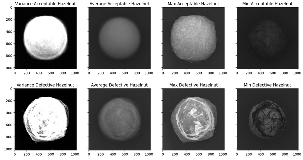
def find_stat_img(full_mat, title, size = (1024, 1024)):
# calculate the average
mean_img = np.mean(full_mat, axis = 0)
mean_img = mean_img.reshape(size)
var_img = np.var(full_mat, axis = 0)
var_img = var_img.reshape(size)
max_img = np.amax(full_mat, axis = 0)
max_img = max_img.reshape(size)
min_img = np.amin(full_mat, axis = 0)
min_img = min_img.reshape(size)
figure, (ax1, ax2, ax3, ax4) = plt.subplots(1, 4, sharey=True, figsize=(15, 15))
ax1.imshow(var_img, vmin=0, vmax=255, cmap='Greys_r')
ax1.set_title(f'Variance {
title}')
ax2.imshow(mean_img, vmin=0, vmax=255, cmap='Greys_r')
ax2.set_title(f'Average {
title}')
ax3.imshow(max_img, vmin=0, vmax=255, cmap='Greys_r')
ax3.set_title(f'Max {
title}')
ax4.imshow(min_img, vmin=0, vmax=255, cmap='Greys_r')
ax4.set_title(f'Min {
title}')
plt.show()
return mean_img, var_img
此处的传参需要根据图片尺寸来调整,这里可以看到简单分析后的效果:
- 模型定义
接下来进行模型的定义,这里直接引用了官方代码:
class CustomVGG(nn.Module):

    def __init__(self, n_classes=2):
        super().__init__()
        self.feature_extractor = models.vgg16(pretrained=True).features[:-1]
        self.classification_head = nn.Sequential(
            nn.MaxPool2d(kernel_size=2, stride=2),
            nn.AvgPool2d(
                kernel_size=(INPUT_IMG_SIZE[0] // 2 ** 5, INPUT_IMG_SIZE[1] // 2 ** 5)
            ),
            nn.Flatten(),
            nn.Linear(
                in_features=self.feature_extractor[-2].out_channels,
                out_features=n_classes,
            ),
        )
        self._freeze_params()

    def _freeze_params(self):
        for param in self.feature_extractor[:23].parameters():
            param.requires_grad = False

    def forward(self, x_in):
        """
        forward
        """
        feature_maps = self.feature_extractor(x_in)
        scores = self.classification_head(feature_maps)

        if self.training:
            return scores

        probs = nn.functional.softmax(scores, dim=-1)

        weights = self.classification_head[3].weight
        weights = (
            weights.unsqueeze(-1)
            .unsqueeze(-1)
            .unsqueeze(0)
            .repeat(
                (
                    x_in.size(0),
                    1,
                    1,
                    INPUT_IMG_SIZE[0] // 2 ** 4,
                    INPUT_IMG_SIZE[0] // 2 ** 4,
                )
            )
        )
        feature_maps = feature_maps.unsqueeze(1).repeat((1, probs.size(1), 1, 1, 1))
        location = torch.mul(weights, feature_maps).sum(axis=2)
        location = F.interpolate(location, size=INPUT_IMG_SIZE, mode="bilinear")

        maxs, _ = location.max(dim=-1, keepdim=True)
        maxs, _ = maxs.max(dim=-2, keepdim=True)
        mins, _ = location.min(dim=-1, keepdim=True)
        mins, _ = mins.min(dim=-2, keepdim=True)
        norm_location = (location - mins) / (maxs - mins)

        return probs, norm_location
接下来需要不断的反复调整参数,来查看模型的表现,此处略去。
- 模型训练
根据定义好的参数训练模型,然后使用测试集查看具体表现。
# model training starts
# Model Training
# Intitalization of DL architechture along with optimizer and loss function
model = CustomVGG()
class_weight = torch.tensor(class_weight).type(torch.FloatTensor).to(DEVICE)
criterion = nn.CrossEntropyLoss(weight=class_weight)
optimizer = optim.Adam(model.parameters(), lr=LR)

# Ipex Optimization
model, optimizer = ipex.optimize(model=model, optimizer=optimizer, dtype=torch.float32)

# Training module
start_time = time.time()
trained_model = train(train_loader, model=model, optimizer=optimizer, criterion=criterion, epochs=EPOCHS,
    device=DEVICE, target_accuracy=TARGET_TRAINING_ACCURACY)
train_time = time.time()-start_time

# Save weights
model_path = f"{

      subset_name}.pt"
torch.save(trained_model.state_dict(), model_path)
3. 评估和量化
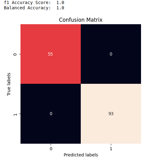
- 模型评估
评估一个模型有多个指标,可以使用evaluate等方法查看。
y_true, y_pred = evaluate(trained_model, test_loader, DEVICE, labels=True)
- 模型量化
在模型训练完成后,可以将其量化导出,这样通过十分简短的代码就可以调用。
from neural_compressor.config import PostTrainingQuantConfig, AccuracyCriterion, TuningCriterion
from neural_compressor import quantization

# INC will not quantize some layers optimized by ipex, such as _IPEXConv2d,
# so we need to create original model object and load trained weights
model = CustomVGG()
model.load_state_dict(torch.load(model_path))
model.to(DEVICE)
model.eval()

# define evaluation function used by INC
def eval_func(model):
    with torch.no_grad():
        y_true = np.empty(shape=(0,))
        y_pred = np.empty(shape=(0,))

        for inputs, labels in train_loader:
            inputs = inputs.to(DEVICE)
            labels = labels.to(DEVICE)
            preds_probs = model(inputs)[0]
            preds_class = torch.argmax(preds_probs, dim=-1)
            labels = labels.to("cpu").numpy()
            preds_class = preds_class.detach().to("cpu").numpy()
            y_true = np.concatenate((y_true, labels))
            y_pred = np.concatenate((y_pred, preds_class))

    return accuracy_score(y_true, y_pred)


# quantize model
conf = PostTrainingQuantConfig(backend='ipex',
                               accuracy_criterion = AccuracyCriterion(
                                   higher_is_better=True,
                                   criterion='relative',
                                   tolerable_loss=0.01))
q_model = quantization.fit(model,
                           conf,
                           calib_dataloader=train_loader,
                           eval_func=eval_func)

# save quantized model
# you can also find a json file saved with quantized model, which saved quantization information for each operator
quantized_model_path = './quantized_models'
if not os.path.exists(quantized_model_path):
    os.makedirs(quantized_model_path)
q_model.save(quantized_model_path)
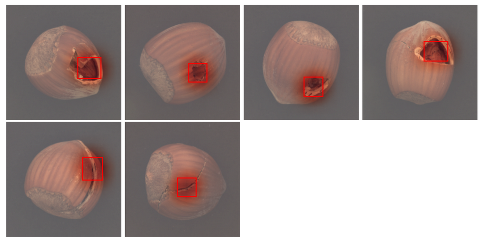
- 模型预测
从指定路径加载模型后就可以开始预测:
q_model.to(DEVICE)
q_model.eval()
q_model = ipex.optimize(q_model)

y_true, y_pred = evaluate(q_model, test_loader, DEVICE, labels=True)
扫描下方二维码,加入CSDN官方粉丝微信群,可以与我直接交流,还有更多福利哦~
