一、回归
训练数据集click.csv如下:
x,y
235,591
216,539
148,413
35,310
85,308
204,519
49,325
25,332
25,332
173,498
191,498
134,392
99,334
117,385
112,387
162,425
272,659
159,427
59,319
198,522
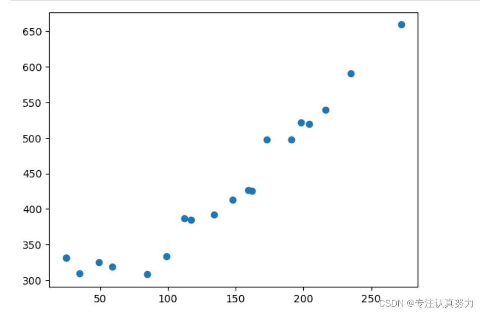
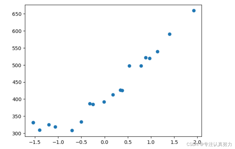
我们的目的是从该数据集中发现一种规律,通过该规律我们可以根据任意给定的y值,预测出x的值。这个过程也被称为学习。
首先我们把这些点在二维坐标系中显示出来,通过图像可以更加直观的发现数据的分布规律。
import numpy as np
import matplotlib.pyplot as plt
# 读入训练数据
train = np.loadtxt('click.csv',delimiter=',',skiprows=1)
train_x = train[:,0]
train_y = train[:,1]
# 绘图
plt.plot(train_x,train_y,'o')
plt.show()
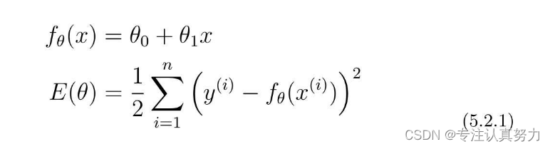
我们把这个数据集的要学习的规律称为fθ(x)。
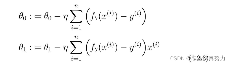
首先把fθ(x)作为一次函数来实现吧。我们要实现下面这样的fθ(x)和目标函数E(θ)。
 对进行θ0和θ1的初始化,用随机值作初始值。
# 参数初始化
theta0 = np.random.rand()
theta1 = np.random.rand()

# 预测函数
def f(x):
    return theta0+theta1*x

# 目标函数
def E(x,y):
    return 0.5*sum((y-f(x))**2)
对训练数据进行预处理:把训练数据变成平均值为0、方差为1的数据。
这个预处理不是必须的,但是做了之后,参数的收敛会更快。这种做法也被称为标准化或者z-score规范化,变换表达式是这样的。µ是训练数据的平均值,σ是标准差。
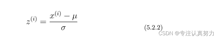
# 标准化
mu = train_x.mean()
sigma = train_x.std()
def standardize(x):
    return (x-mu)/sigma
train_z = standardize(train_x)

plt.plot(train_z,train_y,'o')
plt.show()
可以发现经过标准化后横轴的刻度变小了。
接下来就是去寻找fθ(x)的规律,由于我们假设该数据集具有一次函数的规律。对于一次函数,我们需要从数据集中得到两个参数θ0、θ1,使其能够尽可能经过数据集的所有点。
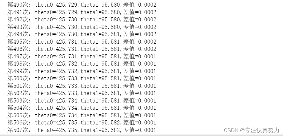
利用梯度下降的方法去寻找使误差函数E(θ)最小的两个参数。
# 学习率
ETA = 1e-3
# 误差的差值
diff = 1
# 更新次数
count = 0
# 重复学习
error = E(train_z,train_y)
while diff > 1e-4:
    # 更新结果保存到临时变量
    tmp0 = theta0 - ETA*np.sum((f(train_z)-train_y))
    tmp1 = theta1 - ETA*np.sum((f(train_z)-train_y)*train_z)
    # 更新参数
    theta0 = tmp0
    theta1 = tmp1
    # 计算与上一次的差值
    current_error = E(train_z,train_y)
    diff = error - current_error
    error = current_error
    # 输出日志
    count += 1
    log = '第{}次:theta0={:.3f},theta1={:.3f},差值={:.4f}'
    print(log.format(count,theta0,theta1,diff))
# 绘图确认
x = np.linspace(-3,3,100)
plt.plot(train_z,train_y,'o')
plt.plot(x,f(x))
plt.show()
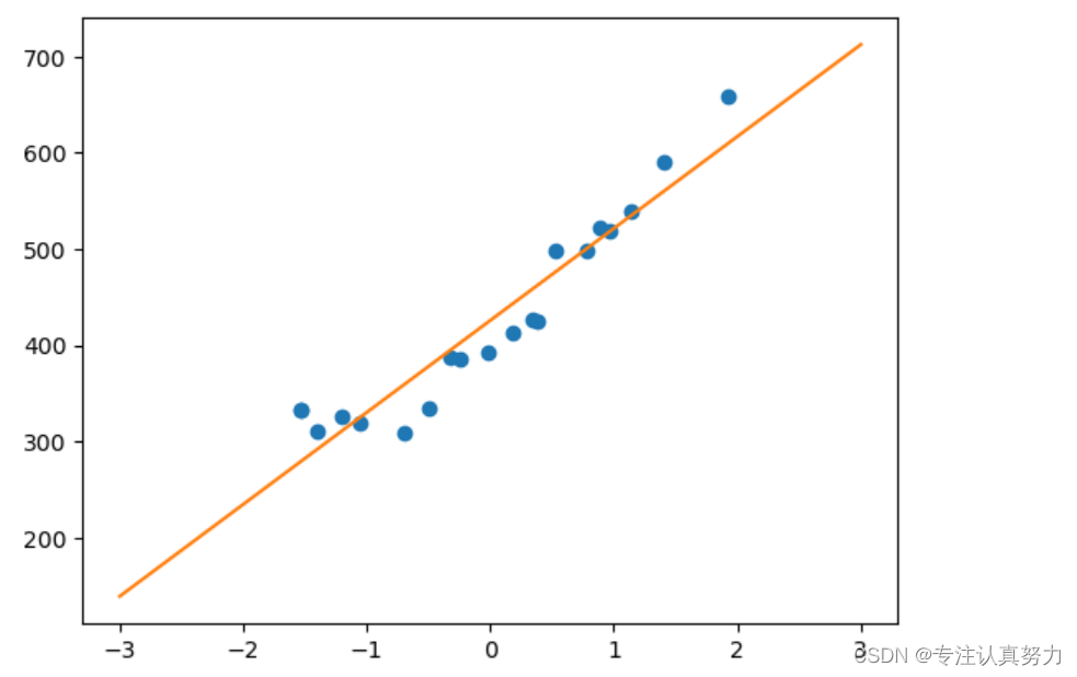
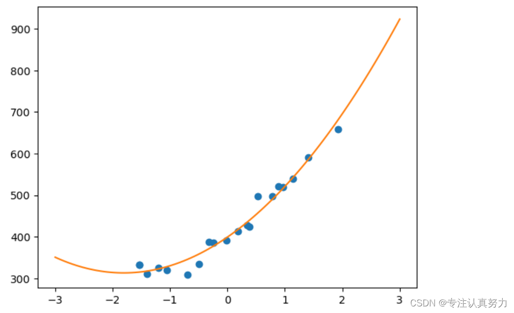
前面我们假设数据集中的规律为一次函数,并对其成功进行了拟合。
实际上,我们也可以假设规律为二次函数。
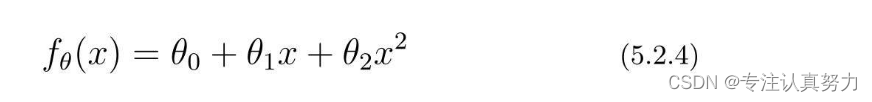
将参数和训练数据都作为向量来处理,可以使计算变得更简单。
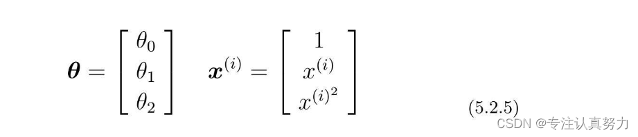
不过由于训练数据有很多,所以我们把1行数据当作1个训练数据,以矩阵的形式来处理会更好。
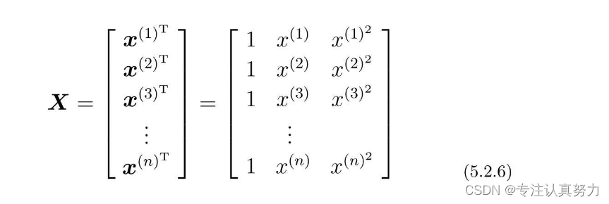
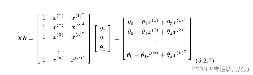
然后,再求这个矩阵与参数向量θ的积。
# 初始化参数
theta = np.random.rand(3)
# 创建训练数据的矩阵
def to_matrix(x):
    return np.vstack([np.ones(x.shape[0]),x,x ** 2]).T
X = to_matrix(train_z)
# 预测函数
def f(x):
    return np.dot(x,theta)
# 误差的差值
diff = 1
# 重复学习
error = E(X,train_y)
while diff > 1e-3:
    # 更新参数
    theta = theta - ETA * np.dot(f(X)-train_y,X)
    # 计算与上一次误差的差值
    current_error = E(X,train_y)
    diff = error -current_error
    error = current_error
x = np.linspace(-3,3,100)
plt.plot(train_z,train_y,'o')
plt.plot(x,f(to_matrix(x)))
plt.show()
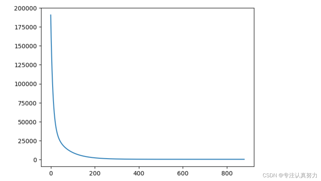
# 均方误差
def MSE(x,y):
    return (1 / x.shape[0]) * np.sum((y-f(x))**2)
# 用随机值初始化参数
theta = np.random.rand(3)
# 均方误差的历史记录
errors = []
# 误差的差值
diff = 1
# 重复学习
errors.append(MSE(X,train_y))
while diff > 1e-3:
    theta = theta - ETA * np.dot(f(X)-train_y,X)
    errors.append(MSE(X,train_y))
    diff = errors[-2]-errors[-1]
# 绘制误差变化图
x = np.arange(len(errors))
plt.plot(x,errors)
plt.show()
二、分类——感知机
训练数据集images1.csv如下:
x1,x2,y
153,432,-1
220,262,-1
118,214,-1
474,384,1
485,411,1
233,430,-1
396,361,1
484,349,1
429,259,1
286,220,1
399,433,-1
403,340,1
252,34,1
497,472,1
379,416,-1
76,163,-1
263,112,1
26,193,-1
61,473,-1
420,253,1
实现步骤:
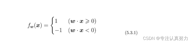
1.首先要初始化感知机的权重,然后实现函数fw(x)。
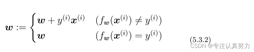
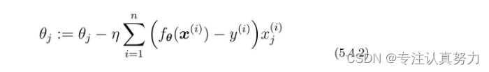
2.接下来只需实现权重的更新表达式。
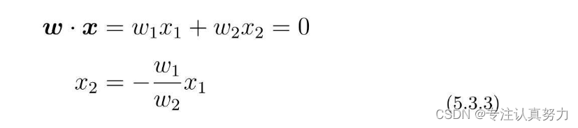
3.使权重向量成为法线向量的直线方程是内积为0的x的集合。所以对它进行移项变形,最终绘出以下表达式的图形即可。
import numpy as np
import matplotlib.pyplot as plt
train = np.loadtxt("data/images1.csv", delimiter=",", skiprows=1)
train_x = train[:, 0:2]
train_y = train[:, 2]
# 权重的初始化
w = np.random.rand(2) # 生成两个符合0-1分布的随机值,以列表形式保存
# 判别函数
def f(x_f):
if np.dot(w, x_f) >= 0:
return 1
else:
return -1
# 重复次数
epoch = 10
# 更新次数
count = 0
# 学习权重
for _ in range(epoch):
for x, y in zip(train_x, train_y):
if f(x) != y:
w = w + y * x
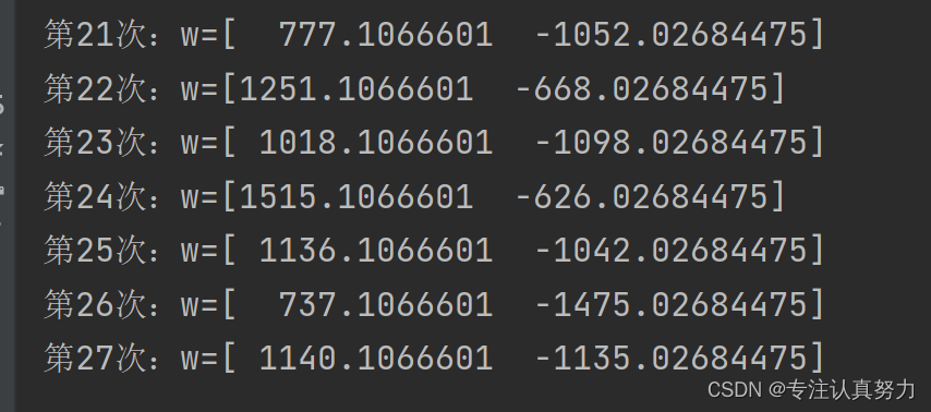
# 输出日志
count += 1
print('第{}次:w={}'.format(count, w))
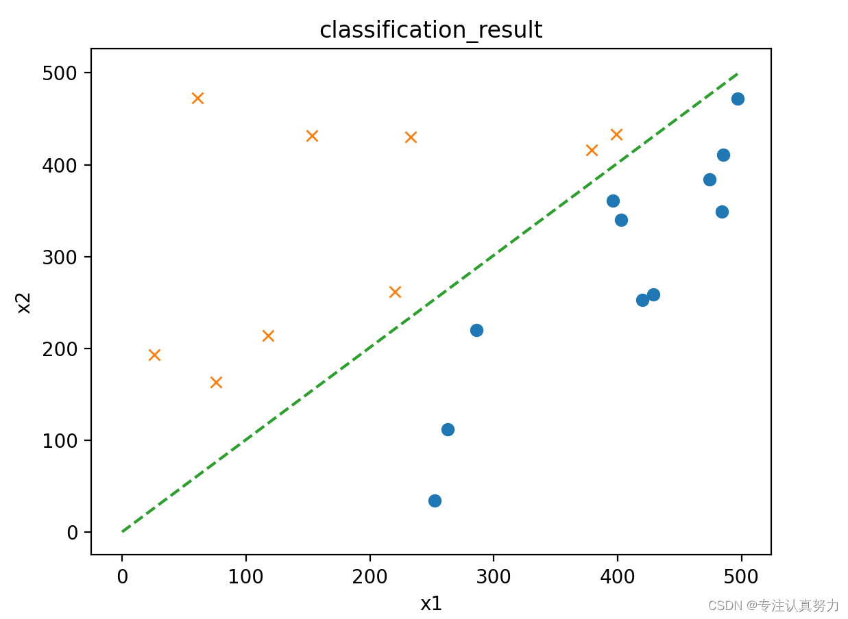
# 绘图
x1 = np.arange(0, 500)
plt.title("classification_result")
plt.xlabel('x1')
plt.ylabel('x2')
plt.plot(train_x[train_y == 1, 0], train_x[train_y == 1, 1], "o")
plt.plot(train_x[train_y == -1, 0], train_x[train_y == -1, 1], "x")
plt.plot(x1, -w[0] / w[1] * x1, linestyle='dashed')
plt.show()
三、分类——逻辑回归
将images1.csv中的-1标签改变为0,得到训练数据集images2.csv如下:
x1,x2,y
153,432,0
220,262,0
118,214,0
474,384,1
485,411,1
233,430,0
396,361,1
484,349,1
429,259,1
286,220,1
399,433,0
403,340,1
252,34,1
497,472,1
379,416,0
76,163,0
263,112,1
26,193,0
61,473,0
420,253,1
实现步骤:
1.首先初始化参数,然后对训练数据标准化吧。x1和x2要分别标准化。另外不要忘了加一个x0列。
2.实现预测函数。

3.接下来是参数更新部分的实现。
4. 将θTx=0变形并加以整理,得到这样的表达式。
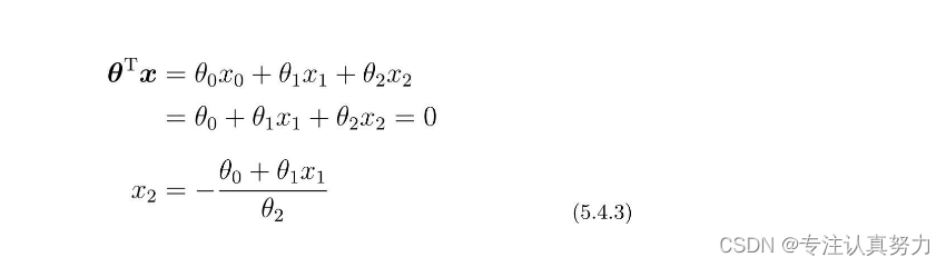
import numpy as np
import matplotlib.pyplot as plt
# 读入训练数据
train = np.loadtxt("data/images2.csv", delimiter=",", skiprows=1)
train_x = train[:, 0:2]
train_y = train[:, 2]
# 参数初始化
theta = np.random.rand(3)
# 标准化
mu = train_x.mean(axis=0)
sigma = train_x.std(axis=0)
def standardize(x):
return (x - mu) / sigma
train_z = standardize(train_x)
# 增加x0
def to_matrix(x):
x0 = np.ones([x.shape[0], 1])
return np.hstack([x0, x])
X = to_matrix(train_z)
# sigmoid 函数
def f(x):
return 1 / (1 + np.exp(-np.dot(x, theta)))
# 分类函数
def classify(x):
return (f(x) >= 0.5).astype(np.int)
# 学习率
ETA = 1e-3
# 重复次数
epoch = 5000
# 更新次数
count = 0
# 重复学习
for _ in range(epoch):
theta = theta - ETA * np.dot(f(X) - train_y, X)
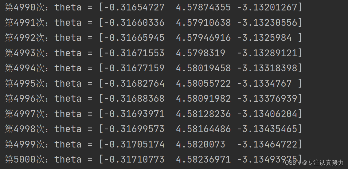
# 日志输出
count += 1
print('第{}次:theta = {}'.format(count, theta))
# 绘图确认
x0 = np.linspace(-2, 2, 100)
plt.title("classification_result")
plt.xlabel('x1')
plt.ylabel('x2')
plt.plot(train_z[train_y == 1, 0], train_z[train_y == 1, 1], 'o')
plt.plot(train_z[train_y == 0, 0], train_z[train_y == 0, 1], 'x')
plt.plot(x0, -(theta[0] + theta[1] * x0) / theta[2], linestyle='dashed')
plt.show()
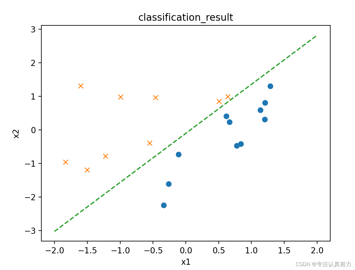
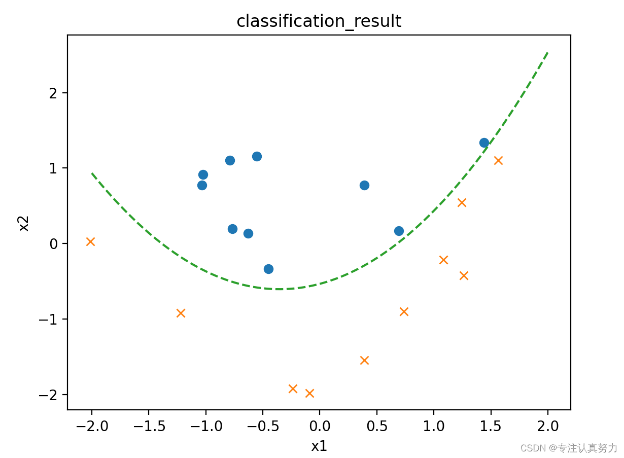
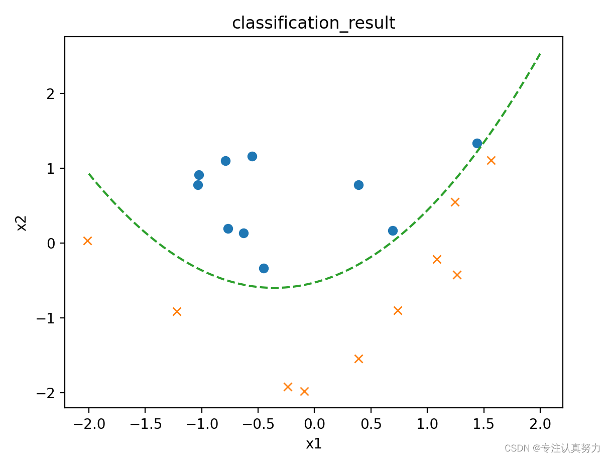
以上数据都可以通过一条直线将其进行分类,我们称之为线性可分的分类问题,对于如下数据,可以发现它们是无法仅仅通过一条直线就可以完成分类。
训练数据集data3.csv如下:
x1,x2,y
0.54508775,2.34541183,0
0.32769134,13.43066561,0
4.42748117,14.74150395,0
2.98189041,-1.81818172,1
4.02286274,8.90695686,1
2.26722613,-6.61287392,1
-2.66447221,5.05453871,1
-1.03482441,-1.95643469,1
4.06331548,1.70892541,1
2.89053966,6.07174283,0
2.26929206,10.59789814,0
4.68096051,13.01153161,1
1.27884366,-9.83826738,1
-0.1485496,12.99605136 ,0
-0.65113893,10.59417745,0
3.69145079,3.25209182,1
-0.63429623,11.6135625,0
0.17589959,5.84139826,0
0.98204409,-9.41271559,1
-0.11094911,6.27900499,0
import numpy as np
import matplotlib.pyplot as plt
# 导入数据集
train = np.loadtxt("data/data3.csv", delimiter=",", skiprows=1)
train_x = train[:, 0:2]
train_y = train[:, 2]
# 参数初始化
theta = np.random.rand(4)
# 标准化
mu = train_x.mean(axis=0)
sigma = train_x.std(axis=0)
def standardize(x):
return (x - mu) / sigma
train_z = standardize(train_x)
# 增加x0和x3
def to_matrix(x):
x0 = np.ones([x.shape[0], 1])
x3 = x[:, 0, np.newaxis] ** 2
return np.hstack([x0, x, x3])
X = to_matrix(train_z)
# sigmoid 函数
def f(x):
return 1 / (1 + np.exp(-np.dot(x, theta)))
# 分类函数
def classify(x):
return (f(x) >= 0.5).astype(np.int)
# 学习率
ETA = 1e-3
# 重复次数
epoch = 2000
# 更新次数
count = 0
# 精度的历史记录
accuracies = []
# 重复学习
for _ in range(epoch):
theta = theta - ETA * np.dot(f(X) - train_y, X)
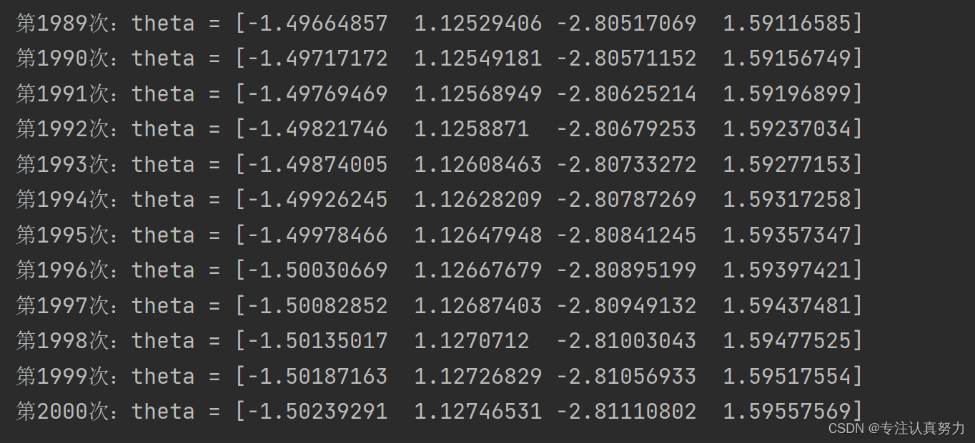
# 日志输出
count += 1
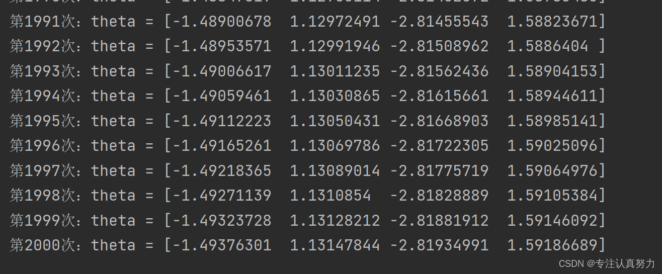
print('第{}次:theta = {}'.format(count, theta))
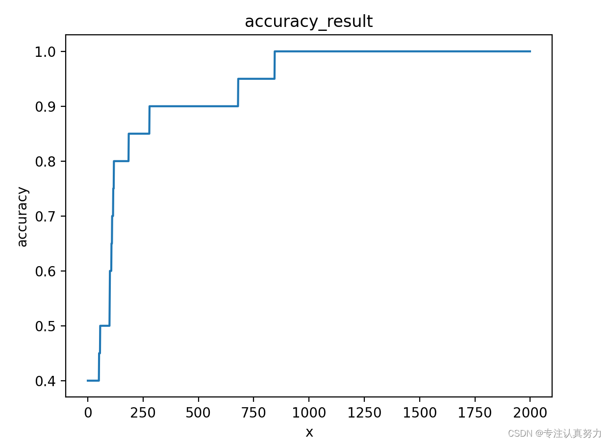
# 计算现在的精度
result = classify(X) == train_y
accuracy = len(result[result == True]) / len(result)
accuracies.append(accuracy)
x1 = np.linspace(-2, 2, 100)
x2 = -(theta[0] + theta[1] * x1 + theta[3] * x1 ** 2) / theta[2]
plt.title("classification_result")
plt.xlabel('x1')
plt.ylabel('x2')
plt.plot(train_z[train_y == 0, 0], train_z[train_y == 0, 1], "o")
plt.plot(train_z[train_y == 1, 0], train_z[train_y == 1, 1], "x")
plt.plot(x1, x2, linestyle='dashed')
plt.show()
x = np.arange(len(accuracies))
plt.plot(x, accuracies)
plt.show()
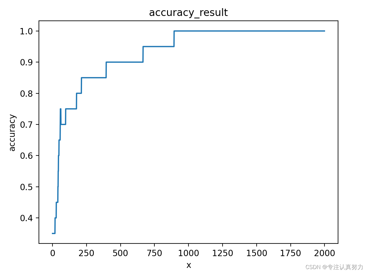
更新参数时,我们选择随机梯度下降的方法进行参数更新。
import numpy as np
import matplotlib.pyplot as plt

# 导入数据集
train = np.loadtxt("data/data3.csv", delimiter=",", skiprows=1)
train_x = train[:, 0:2]
train_y = train[:, 2]

# 参数初始化
theta = np.random.rand(4)

# 标准化
mu = train_x.mean(axis=0)
sigma = train_x.std(axis=0)


def standardize(x):
    return (x - mu) / sigma


train_z = standardize(train_x)


# 增加x0和x3
def to_matrix(x):
    x0 = np.ones([x.shape[0], 1])
    x3 = x[:, 0, np.newaxis] ** 2
    return np.hstack([x0, x, x3])


X = to_matrix(train_z)


# sigmoid 函数
def f(x):
    return 1 / (1 + np.exp(-np.dot(x, theta)))


# 分类函数
def classify(x):
    return (f(x) >= 0.5).astype(np.int)


# 学习率
ETA = 1e-3

# 重复次数
epoch = 2000

# 更新次数
count = 0

# 精度的历史记录
accuracies = []

# 重复学习
for _ in range(epoch):
    # 使用随机梯度下降法更新参数
    p = np.random.permutation(X.shape[0])
    for x, y in zip(X[p, :], train_y[p]):
        theta = theta - ETA * (f(x) - y) * x
    # 日志输出
    count += 1
    print('第{}次:theta = {}'.format(count, theta))
    # 计算现在的精度
    result = classify(X) == train_y
    accuracy = len(result[result == True]) / len(result)
    accuracies.append(accuracy)

x1 = np.linspace(-2, 2, 100)
x2 = -(theta[0] + theta[1] * x1 + theta[3] * x1 ** 2) / theta[2]
plt.title("classification_result")
plt.xlabel('x1')
plt.ylabel('x2')
plt.plot(train_z[train_y == 0, 0], train_z[train_y == 0, 1], "o")
plt.plot(train_z[train_y == 1, 0], train_z[train_y == 1, 1], "x")
plt.plot(x1, x2, linestyle='dashed')
plt.show()

x = np.arange(len(accuracies))
plt.title("accuracy_result")
plt.xlabel('x')
plt.ylabel('accuracy')
plt.plot(x, accuracies)
plt.show()
四、正则化
import numpy as np
import matplotlib.pyplot as plt
# 真正的函数
def g(x):
return 0.1 * (x ** 3 + x ** 2 + x)
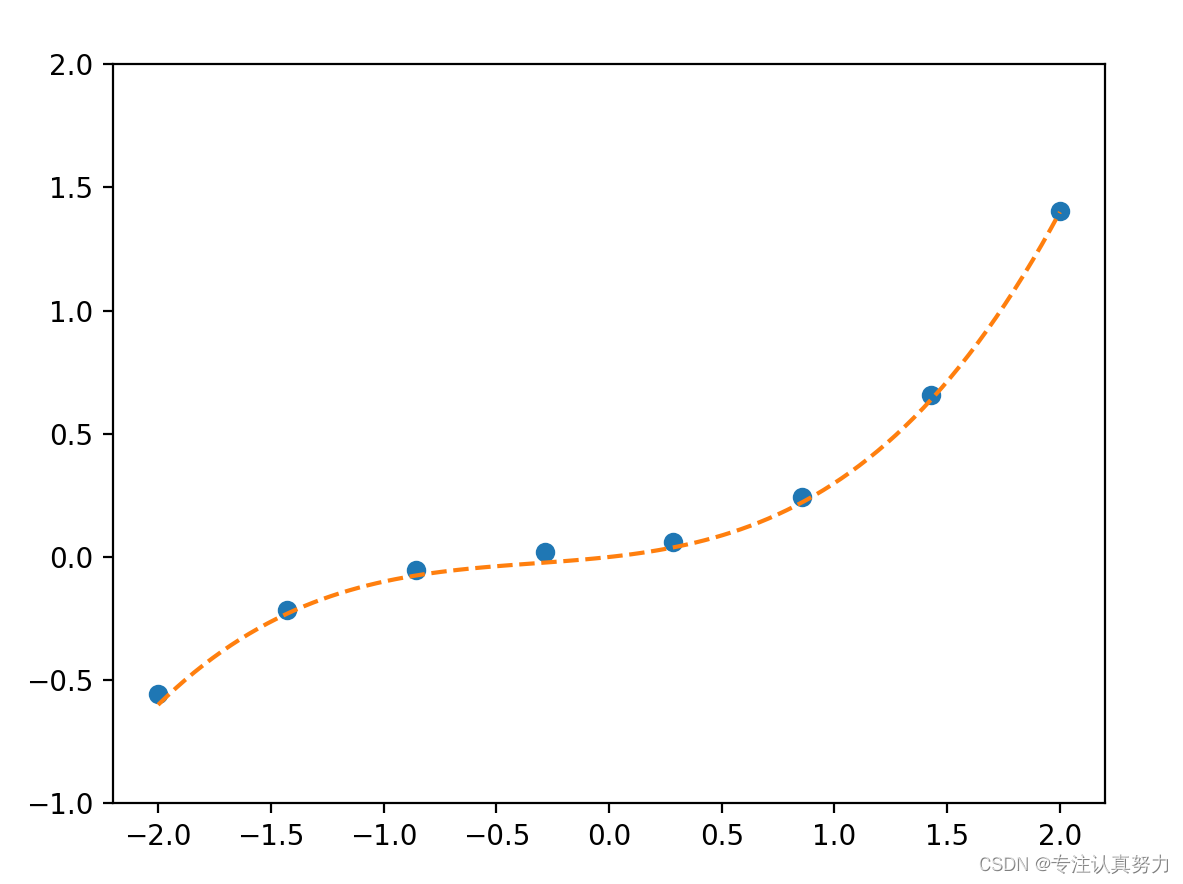
# 随意准备一些向真正的函数加入了一点噪声的训练数据
train_x = np.linspace(-2, 2, 8)
train_y = g(train_x) + np.random.rand(train_x.size) * 0.05
# 绘图确认
plt.plot(train_x, train_y, 'o')
x = np.linspace(-2, 2, 100)
plt.plot(x, g(x), linestyle="dashed")
plt.ylim(-1, 2)
plt.show()
# 标准化
mu = train_x.mean()
sigma = train_x.std()
def standardize(x):
return (x - mu) / sigma
train_z = standardize(train_x)
# 创建训练数据的矩阵
def to_matrix(x):
return np.vstack([np.ones(x.size),
x,
x ** 2,
x ** 3,
x ** 4,
x ** 5,
x ** 6,
x ** 7,
x ** 8,
x ** 9,
x ** 10]).T
X = to_matrix(train_z)
# 参数初始化
theta = np.random.randn(X.shape[1])
# 预测函数
def f(x):
return np.dot(x, theta)
# 目标函数
def E(x, y):
return 0.5 * np.sum((y - f(x)) ** 2)
# 学习率
ETA = 1e-4
# 误差
diff = 1
# 重复学习
error = E(X, train_y)
while diff > 1e-6:
theta = theta - ETA * np.dot(f(X) - train_y, X)
current_error = E(X, train_y)
diff = error - current_error
error = current_error
# 对结果绘图
z = standardize(x)
plt.plot(train_z, train_y, 'o')
plt.plot(z, f(to_matrix(z)))
plt.show()
# 保存未正则化的参数,然后再次参数初始化
theta1 = theta
theta = np.random.randn(X.shape[1])
# 正则化常量
LAMBDA = 1
# 误差
diff = 1
# 重复学习(包含正则化项)
error = E(X, train_y)
while diff > 1e-6:
# 正则化项。偏置项不适合正则化,所以为0
reg_term = LAMBDA * np.hstack([0, theta[1:]])
# 应用正则化项,更新参数
theta = theta - ETA * (np.dot(f(X) - train_y, X) + reg_term)
current_error = E(X, train_y)
diff = error - current_error
error = current_error
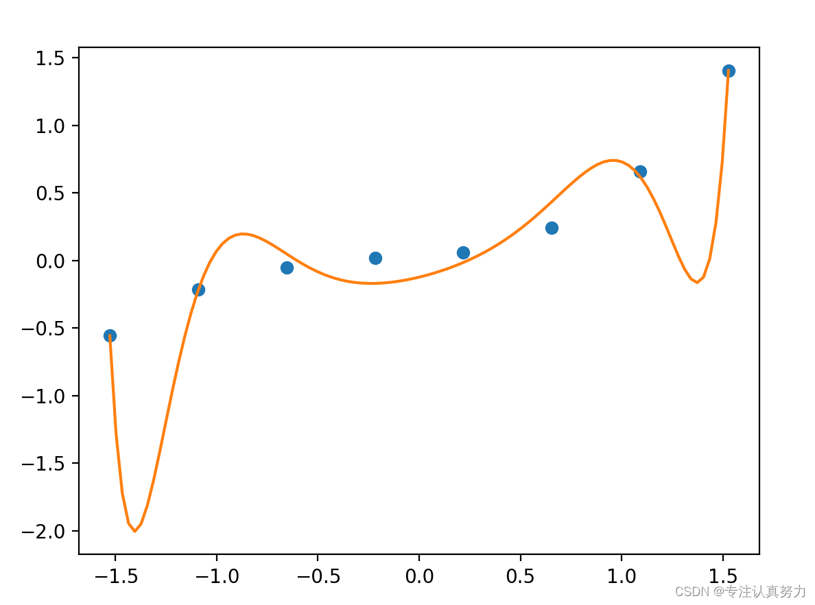
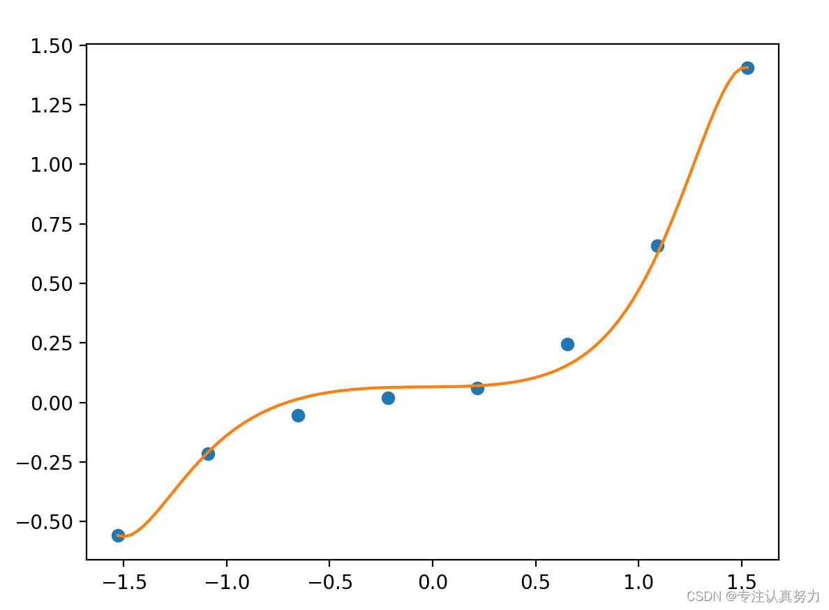
# 对结果绘图
plt.plot(train_z, train_y, 'o')
plt.plot(z, f(to_matrix(z)))
plt.show()
theta2 = theta
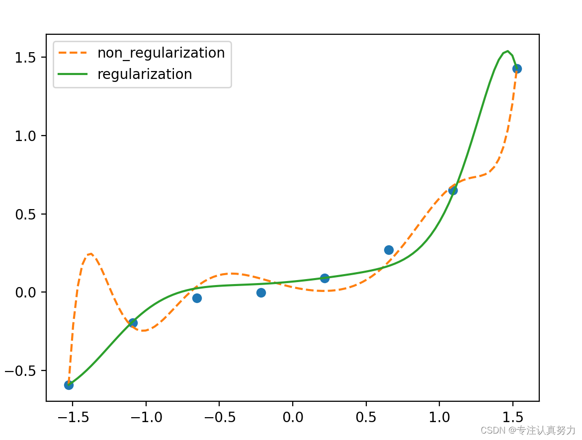
plt.plot(train_z, train_y, 'o')
# 画出未正则化的结果
theta = theta1
plt.plot(z, f(to_matrix(z)), linestyle='dashed', label="non_regularization")
# 画出正则化的结果
theta = theta2
plt.plot(z, f(to_matrix(z)), label="regularization")
plt.legend()
plt.show()
我们利用一个真正的函数来生成数据,并在其中添加随机的噪声,以对现实进行模拟。
不进行正则化处理的学习效果。
进行正则化处理的学习结果。
两者间的对比。