边写代码边学习之全连接Dense

1. 全连接原理

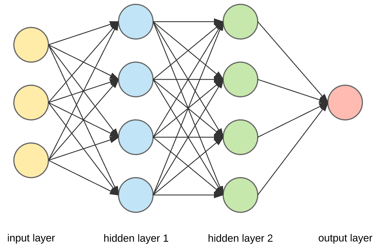
全连接神经网络（Fully Connected Neural Network）是一种最基本的神经网络结构，也被称为多层感知器（Multilayer Perceptron，MLP）。其原理是模拟人脑神经元之间的连接方式，通过多个层次的神经元组成，每个神经元都与上一层和下一层的所有神经元相连接。

全连接神经网络的原理如下：

1. 输入层（Input Layer）：接受输入数据，每个输入特征对应一个输入节点。

2. 隐藏层（Hidden Layer）：位于输入层和输出层之间，可以包含多个层。每个隐藏层由多个神经元组成，每个神经元与上一层的所有神经元相连接，并带有权重值。

3. 输出层（Output Layer）：输出神经网络的预测结果，通常对应问题的类别或数值。

4. 权重（Weights）：每个连接都有一个权重值，表示连接的强度。权重值在网络训练过程中更新，以使神经网络能够学习到合适的特征表示和模式。

5. 偏置（Biases）：每个神经元都带有一个偏置项，它可以看作是神经元的激活阈值。偏置可以调整神经元是否被激活。

6. 激活函数（Activation Function）：位于每个神经元中，用于引入非线性性，允许神经网络学习复杂的函数映射。常见的激活函数包括Sigmoid、ReLU、tanh等。

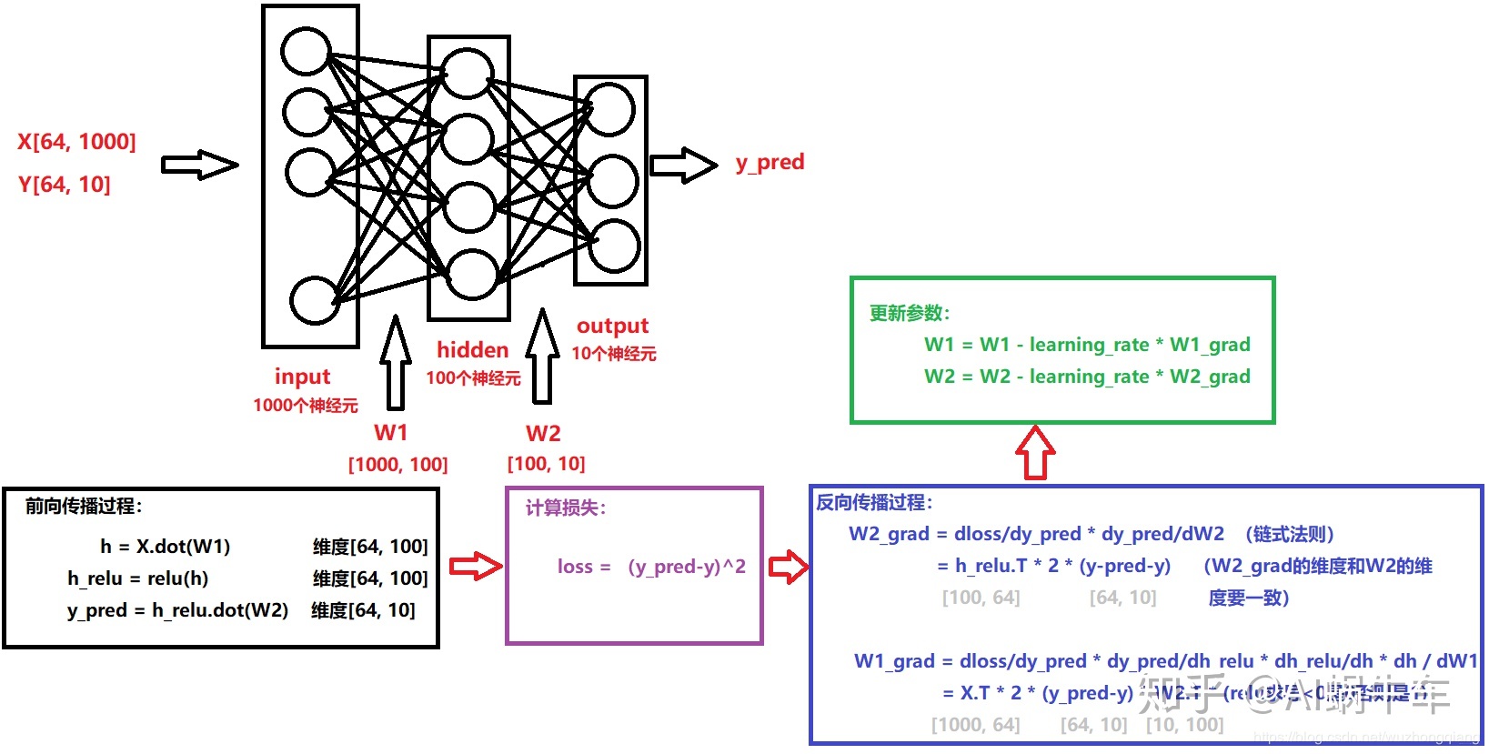
 训练全连接神经网络的过程一般通过反向传播算法（Backpropagation）来实现。它包括前向传播（从输入到输出）计算预测结果，并计算预测值与真实值之间的误差；然后通过反向传播计算梯度并更新网络中的权重和偏置，以最小化误差函数。这个过程会不断迭代，直到网络达到较好的预测性能。

缺点：

全连接神经网络在处理大规模数据时，可能会面临过拟合、计算资源消耗大等问题。为了解决这些问题，人们开发了更复杂的神经网络结构，例如卷积神经网络（CNN）和循环神经网络（RNN），它们在特定领域表现出色。

2. tf.keras.layers.Dense 方法以及参数的详细介绍

tf.keras.layers.Dense(
    units,
    activation=None,
    use_bias=True,
    kernel_initializer="glorot_uniform",
    bias_initializer="zeros",
    kernel_regularizer=None,
    bias_regularizer=None,
    activity_regularizer=None,
    kernel_constraint=None,
    bias_constraint=None,
    **kwargs
)

参数

• units：正整数，输出空间的维数。
• activation：要使用的激活函数。 如果您未指定任何内容，则不会应用任何激活（即“线性(linear)”激活：a(x) = x）。
• use_bias：布尔值，该层是否使用偏置向量。
• kernel_initializer：内核权重矩阵的初始化器。
• bias_initializer：偏置向量的初始化器。
• kernel_regularizer：应用于内核权重矩阵的正则化函数。
• bias_regularizer：应用于偏差向量的正则化函数。
• Activity_regularizer：应用于层输出的正则化函数（其“激活”）。
• kernel_constraint：应用于内核权重矩阵的约束函数。
• bias_constraint：应用于偏置向量的约束函数。

只是常规的密集连接（regular densely-connected NN）的神经网络层。

Dense 实现操作：output = activation(dot(input, kernel) + bias)，其中激活（activation）是作为激活参数传递的逐元素（element-wise）激活函数，内核（kernal）是由层创建的权重矩阵(weights matrix)，偏差(bias)是由层创建的偏差向量（仅当 use_bias 为 True 时适用）。 这些都是Dense的属性。

注意：如果该层的输入的秩(rank)大于 2，则 Dense 会沿着输入的最后一个轴和内核的轴 0 计算输入和内核之间的点积（使用 tf.tensordot）。 例如，如果输入的维度为 (batch_size, d0, d1)，那么我们创建一个形状为 (d1,units) 的内核，并且内核kernal沿输入的axis 2 对形状为 (1, 1, d1) 的每个子张量进行操作（有 batch_size * d0 这样的子张量）。 这种情况下的输出将具有形状（batch_size，d0，units）。

此外，层的属性在调用一次后就无法修改（可trainable属性除外）。 当传递流行的 kwarg input_shape 时，keras 将创建一个输入层插入到当前层之前。 这可以被视为等同于显式定义一个InputLayer。

Input Shape

N 维张量(N-D tensor)，shape为：(batch_size, ..., input_dim)。 最常见的情况是形状为 (batch_size, input_dim) 的 2D 输入。

Output Shape

N 维张量(N-D tensor)，shape为：（batch_size，...，units）。 例如，对于shape为（batch_size，input_dim）的 2D 输入，输出将具有形状（batch_size，units）。

3. 例子代码

3.1. 一层Dense模型

建一个只用Dense搭建的模型。输入是20，输出是10. 激活函数是relu.默认是没有激活函数。权重矩阵的shape是（20， 10）。偏置的shape是（10）.  权重参数= 20 x 10 +10

def simple_dense_layer():
    # Create a dense layer with 10 output neurons and input shape of (None, 20)
    model = tf.keras.Sequential([
     keras.layers.Dense(units=10, input_shape=(20,), activation = 'relu')
    ]);
    # Print the summary of the dense layer
    print(model.summary())

if __name__ == '__main__':
    simple_dense_layer()

输出：

Model: "sequential"
_________________________________________________________________
 Layer (type)                Output Shape              Param #   
=================================================================
 dense (Dense)               (None, 10)                210       
                                                                 
=================================================================
Total params: 210
Trainable params: 210
Non-trainable params: 0
_________________________________________________________________

3.2. 多层Dense的模型

三次Dense构建的模型。前两层的激活函数是relu。最后一层是softmax。

def multi_Layer_perceptron():
    input_dim = 20
    output_dim = 5

    # Create a simple MLP with 2 hidden dense layers
    model = tf.keras.Sequential([
        tf.keras.layers.Dense(units=64, activation='relu', input_shape=(input_dim,)),
        tf.keras.layers.Dense(units=32, activation='relu'),
        tf.keras.layers.Dense(units=output_dim, activation='softmax')
    ])

    # Print the model summary
    print(model.summary())
if __name__ == '__main__':
    multi_Layer_Perceptron()

输出

---

Model: "sequential"
_________________________________________________________________
 Layer (type)                Output Shape              Param #   
=================================================================
 dense (Dense)               (None, 64)                1344      
                                                                 
 dense_1 (Dense)             (None, 32)                2080      
                                                                 
 dense_2 (Dense)             (None, 5)                 165       
                                                                 
=================================================================
Total params: 3,589
Trainable params: 3,589
Non-trainable params: 0
_________________________________________________________________

3.3. 查看权重矩阵以及修改权重矩阵和偏置。

定义一个Dense层。输入一组数据使得Dense初始化其权重矩阵和偏置。然后打印权重矩阵和偏置。你会发现都是-1到1之间的随机数字。

def change_weight():
    # Create a simple Dense layer
    dense_layer = keras.layers.Dense(units=5, activation='relu', input_shape=(10,))

    # Simulate input data (batch size of 1 for demonstration)
    input_data = tf.ones((1, 10))

    # Pass the input data through the layer to initialize the weights and biases
    _ = dense_layer(input_data)

    # Access the weights and biases of the dense layer
    weights, biases = dense_layer.get_weights()

    # Print the initial weights and biases
    print("Initial Weights:")
    print(weights)
    print("Initial Biases:")
    print(biases)

输出

Initial Weights:
[[-0.11511135  0.32900262 -0.1294617  -0.03869444 -0.03002286]
 [-0.24887764  0.20832229  0.48636192  0.09694523 -0.0915786 ]
 [-0.22499037 -0.1025297   0.25898546  0.5259896  -0.19001997]
 [-0.28182945 -0.38635993  0.39958888  0.44975716 -0.21765932]
 [ 0.418611   -0.56121594  0.27648276 -0.5158085   0.5256552 ]
 [ 0.34709007 -0.10060292  0.4056484   0.6316313   0.12976009]
 [ 0.40947527 -0.2114836   0.38547724 -0.1086036  -0.29271656]
 [-0.30581984 -0.14133212 -0.11076003  0.36882895  0.3007568 ]
 [-0.45729238  0.16293162  0.11780071 -0.31189078 -0.00128847]
 [-0.46115184  0.18393213 -0.08268476 -0.5187934  -0.608922  ]]
Initial Biases:
[0. 0. 0. 0. 0.]

根据权重矩阵的shape和偏置的shape把他们分别改为1和0. 然后设置Dense里的权重矩阵和偏置。之后，输入一组数据，得到一组输出。你可以根据我们上面的理论手动计算一下然后验证一下是不是最后是相同。

    # Modify the weights and biases (for demonstration purposes)
    new_weights = tf.ones_like(weights)  # Set all weights to 1
    new_biases = tf.zeros_like(biases)  # Set all biases to 0

    # Set the modified weights and biases back to the dense layer
    dense_layer.set_weights([new_weights, new_biases])

    # Access the weights and biases again after modification
    weights, biases = dense_layer.get_weights()

    # Print the modified weights and biases
    print("Modified Weights:")
    print(weights)
    print("Modified Biases:")
    print(biases)

    input_data = tf.constant([[1,1,3,1,2,1,1,1,1,2]])

    output = dense_layer(input_data)

    print(output)

输出

Modified Weights:
[[1. 1. 1. 1. 1.]
 [1. 1. 1. 1. 1.]
 [1. 1. 1. 1. 1.]
 [1. 1. 1. 1. 1.]
 [1. 1. 1. 1. 1.]
 [1. 1. 1. 1. 1.]
 [1. 1. 1. 1. 1.]
 [1. 1. 1. 1. 1.]
 [1. 1. 1. 1. 1.]
 [1. 1. 1. 1. 1.]]
Modified Biases:
[0. 0. 0. 0. 0.]
tf.Tensor([[14. 14. 14. 14. 14.]], shape=(1, 5), dtype=float32)

3.4. 加一个自定义的激活函数

自定义一个激活函数，这个函数非常简单，就是输入值做平方。然后设置自定义权重矩阵和偏置给Dense层，输入自己定义的数据，最后验证结果是不是和介绍的理论是一样。

def custom_Activation_Function():
    def custom_activation(x):
        return tf.square(x)

    dense_layer = keras.layers.Dense(units=2, activation=custom_activation, input_shape=(4,))

    weights = tf.ones((4,2))
    biases = tf.ones((2))


    input_data = tf.ones((1, 4))
    _ = dense_layer(input_data)
    dense_layer.set_weights([weights, biases])

    # Print the modified weights and biases
    print("Modified Weights:")
    print(dense_layer.get_weights()[0])
    print("Modified Biases:")
    print(dense_layer.get_weights()[1])

    input_data = tf.constant([[1, 2, 3, 1]])
    output = dense_layer(input_data)

    print(output)


if __name__ == '__main__':
    custom_Activation_Function()

输出

Modified Weights:
[[1. 1.]
 [1. 1.]
 [1. 1.]
 [1. 1.]]
Modified Biases:
[1. 1.]
tf.Tensor([[64. 64.]], shape=(1, 2), dtype=float32)

3.5. 训练一个模型可以实现具体某个函数

假如我有一个函数：. 我们想让我们模型可以实现它。下面就是实现这个函数的代码。

def certain_function_implementation():
    import numpy as np
    from keras.models import Sequential
    from keras.layers import Dense

    # Generate random data for training
    np.random.seed(42)
    x_train = np.random.rand(1000, 2)  # 100 samples with 2 features (x1 and x2)
    y_train = 2 * x_train[:, 0] + 3 * x_train[:, 1] + np.random.randn(1000) * 0.1 + 4

    # Build the neural network
    model = Sequential()
    model.add(Dense(1, input_shape=(2,), name = 'dense_layer'))

    # Compile the model
    model.compile(optimizer='adam', loss='mean_squared_error')

    # Train the model
    epochs = 400
    model.fit(x_train, y_train, epochs=epochs)

    # Generate random data for testing
    x_test = np.array([[1, 1], [2, 3], [3, 4], [4, 5], [5, 6]])

    # Test the model with the new data
    y_pred = model.predict(x_test)
    print("Predicted outputs:")
    print(y_pred.flatten())
    print(model.get_layer("dense_layer").get_weights())


if __name__ == '__main__':
    certain_function_implementation()

输出结果。 可以看到Dense里的权重参数是：2.0018072， 2.989778，4.005859， 已经靠近我们想要的函数了，我们期望的参数应该是2，3，4. 预测的结果也很理想。误差不会超过0.1.

.....
3Epoch 398/400
32/32 [==============================] - 0s 3ms/step - loss: 0.0095
Epoch 399/400
32/32 [==============================] - 0s 2ms/step - loss: 0.0095
Epoch 400/400
32/32 [==============================] - 0s 3ms/step - loss: 0.0096
1/1 [==============================] - 0s 34ms/step
Predicted outputs:
[ 8.997444 16.978807 21.970394 26.961979 31.953564]
[array([[2.0018072],
       [2.989778 ]], dtype=float32), array([4.005859], dtype=float32)]