LBP学习笔记（1）--- 详解原始模式特征（代码实现）

一.简述LBP算子和LBP原始模式

LBP（Local Binary Pattern）算子是一种用于纹理描述的局部图像特征，由T.Ojala， M.Pietikäinen和D.Harwood在1994年提出。LBP算子通过对图像中每个像素与其周围邻域像素对比，统计邻域像素灰度值大于或等于中心像素的个数，并将统计结果转化为二进制码，用于表示该像素的局部特征。

LBP算子具有灰度不变性和旋转不变性等优点，并且可以快速计算，被广泛应用于人脸识别、纹理分类、行人检测等领域。基于LBP算子的改进，如旋转不变LBP、多尺度LBP等算法也相继被提出。

LBP原始模式是指在LBP算子中，每个像素的二进制编码不包括自己本身，在其周围的8个邻域像素中，统计比其强度值大或等于其强度值的像素总数，将这些像素存储成一个二进制码（对应8位二进制数），最终得到的二进制码即为该像素的LBP原始模式。对于一个3*3邻域的像素集合，共有256种不同的LBP模式（包括全0和全1模式）。

LBP原始模式是LBP算子最基本的形式，在人脸识别、纹理分类等领域有广泛应用。LBP算子具有灰度不变性和旋转不变性等优点，并且可以快速计算，被认为是一种简单、有效的纹理特征描述符。

二.代码实现（关键函数及完整代码）

1.遍历像素，获取原始模式特征

def lbp_basic(self, image_array):
    basic_array = np.zeros(image_array.shape, np.uint8)
    width = image_array.shape[0]
    height = image_array.shape[1]
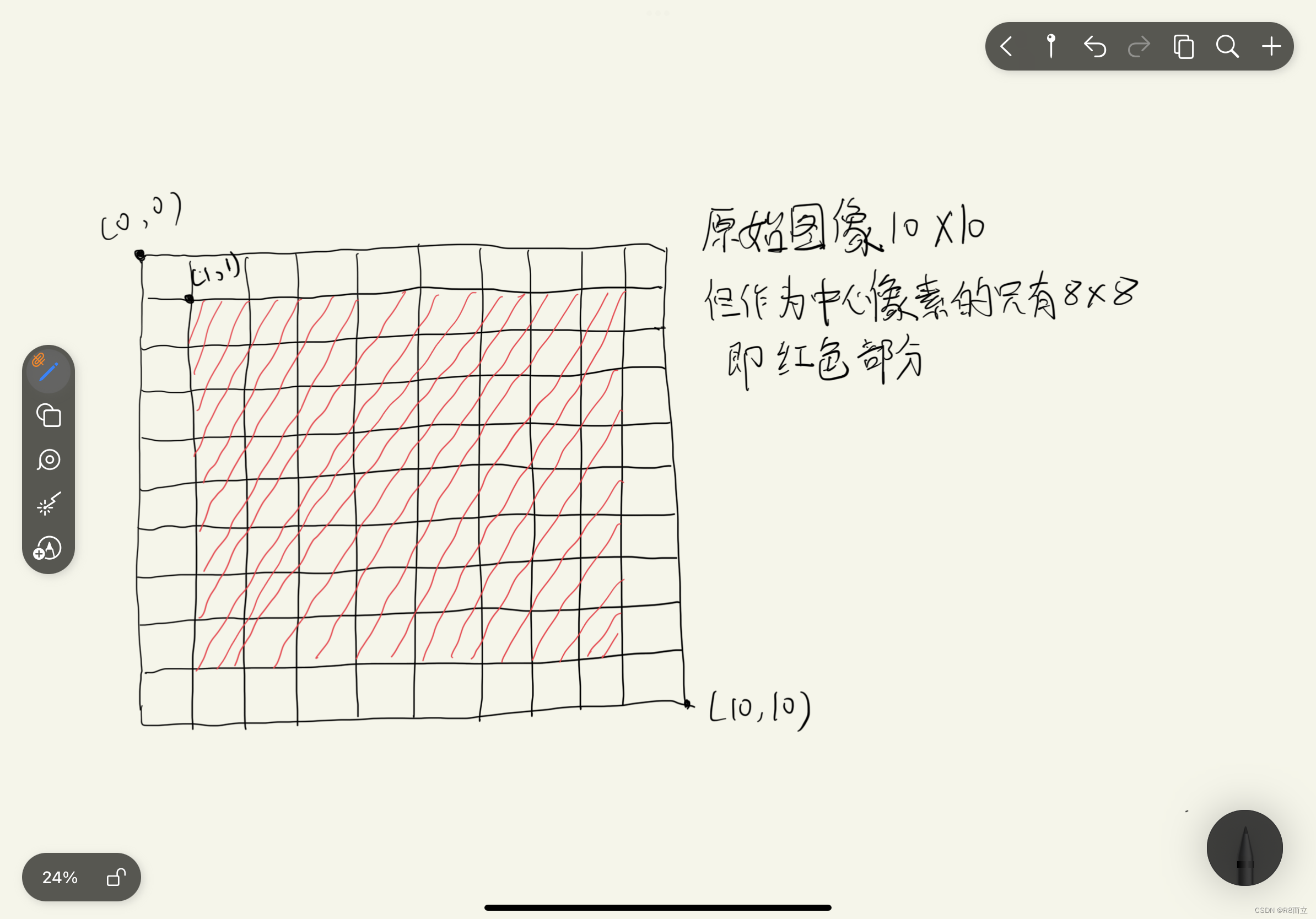
    for i in range(1, width - 1):
        for j in range(1, height - 1):
            sum = self.calute_basic_lbp(image_array, i, j)[1]
            basic_array[i, j] = sum
    return basic_array

先创建一个等大小的全0矩阵，再从图像除去外围一圈后开始遍历，获取到原始模式特征后赋值到刚刚创建的矩阵对应的位置，返回矩阵

2.计算LBP原始模式特征

# 图像的LBP原始特征计算算法：将图像指定位置的像素与周围8个像素比较
# 比中心像素大的点赋值为1，比中心像素小的赋值为0，返回得到的二进制序列
def calute_basic_lbp(self, image_array, i, j):
    sum = []
    num = 0
    if image_array[i - 1, j - 1] > image_array[i, j]:
        sum.append(1)
        num += 2**0
    else:
        sum.append(0)
    if image_array[i - 1, j] > image_array[i, j]:
        sum.append(1)
        num += 2 ** 1
    else:
        sum.append(0)
    if image_array[i - 1, j + 1] > image_array[i, j]:
        sum.append(1)
        num += 2 ** 2
    else:
        sum.append(0)
    if image_array[i, j - 1] > image_array[i, j]:
        sum.append(1)
        num += 2 ** 3
    else:
        sum.append(0)
    if image_array[i, j + 1] > image_array[i, j]:
        sum.append(1)
        num += 2 ** 4
    else:
        sum.append(0)
    if image_array[i + 1, j - 1] > image_array[i, j]:
        sum.append(1)
        num += 2 ** 5
    else:
        sum.append(0)
    if image_array[i + 1, j] > image_array[i, j]:
        sum.append(1)
        num += 2 ** 6
    else:
        sum.append(0)
    if image_array[i + 1, j + 1] > image_array[i, j]:
        sum.append(1)
        num += 2 ** 7
    else:
        sum.append(0)
    return sum,num

历到的像素八邻域的八个像素值和该像素值比较，若大则为1，否则为0。

sum列表储存的是从该像素点的左上角开始顺时针方向的八个像素值与中心像素即该像素的比较结果，是一个二进制的序列，如 [0,0,1,0,1,1,0,1]

num是sum旋转180度后的十进制数。如：sum=[0,0,1,0,1,1,0,1]，则 sum 旋转180度后为[1,0,1,1,0,1,0,0]，num的值就是[1,0,1,1,0,1,0,0]的十进制数，也是该像素点的原始模式特征

在这里直接计算它的特征值，可以提高代码运行的速度

3.绘制直方图

def show_hist(self, img_array, im_bins, im_range):
    # 直方图的x轴是灰度值,y轴是图片中具有同一个灰度值的点的数目, [img_array]原图像图像格式为uint8或ﬂoat32,[0]0表示灰度,None无掩膜
    hist = cv2.calcHist([img_array], [0], None, im_bins, im_range)
    hist = cv2.normalize(hist, hist).flatten()  # 对计算出来的直方图数据进行归一化处理，并将结果扁平化为1D数组
    # print(hist)
    plt.plot(hist, color='r')
    plt.xlim(im_range)  # 设置X轴的取值范围
    plt.show()

4.完整代码

import numpy as np
import cv2
from PIL import Image
from pylab import *

class LBP:

    # 图像的LBP原始特征计算算法：将图像指定位置的像素与周围8个像素比较
    # 比中心像素大的点赋值为1，比中心像素小的赋值为0，返回得到的二进制序列
    def calute_basic_lbp(self, image_array, i, j):
        sum = []
        num = 0
        if image_array[i - 1, j - 1] > image_array[i, j]:
            sum.append(1)
            num += 2**0
        else:
            sum.append(0)
        if image_array[i - 1, j] > image_array[i, j]:
            sum.append(1)
            num += 2 ** 1
        else:
            sum.append(0)
        if image_array[i - 1, j + 1] > image_array[i, j]:
            sum.append(1)
            num += 2 ** 2
        else:
            sum.append(0)
        if image_array[i, j - 1] > image_array[i, j]:
            sum.append(1)
            num += 2 ** 3
        else:
            sum.append(0)
        if image_array[i, j + 1] > image_array[i, j]:
            sum.append(1)
            num += 2 ** 4
        else:
            sum.append(0)
        if image_array[i + 1, j - 1] > image_array[i, j]:
            sum.append(1)
            num += 2 ** 5
        else:
            sum.append(0)
        if image_array[i + 1, j] > image_array[i, j]:
            sum.append(1)
            num += 2 ** 6
        else:
            sum.append(0)
        if image_array[i + 1, j + 1] > image_array[i, j]:
            sum.append(1)
            num += 2 ** 7
        else:
            sum.append(0)
        return sum,num

    # 获取图像的LBP原始模式特征
    def lbp_basic(self, image_array):
        basic_array = np.zeros(image_array.shape, np.uint8)
        width = image_array.shape[0]
        height = image_array.shape[1]
        for i in range(1, width - 1):
            for j in range(1, height - 1):
                sum = self.calute_basic_lbp(image_array, i, j)[1]
                basic_array[i, j]=sum
        return basic_array

    # 绘制指定维数和范围的图像灰度归一化统计直方图
    def show_hist(self, img_array, im_bins, im_range):
        # 直方图的x轴是灰度值,y轴是图片中具有同一个灰度值的点的数目, [img_array]原图像图像格式为uint8或ﬂoat32,[0]0表示灰度,None无掩膜
        hist = cv2.calcHist([img_array], [0], None, im_bins, im_range)
        hist = cv2.normalize(hist, hist).flatten()  # 对计算出来的直方图数据进行归一化处理，并将结果扁平化为1D数组
        # print(hist)
        plt.plot(hist, color='r')
        plt.xlim(im_range)  # 设置X轴的取值范围
        plt.show()

    # 绘制图像原始LBP特征的归一化统计直方图
    def show_basic_hist(self, img_array):
        self.show_hist(img_array, [256], [0, 256])

    # 显示图像
    def show_image(self, image_array):
        plt.imshow(image_array, cmap='Greys_r')
        plt.show()

if __name__ == '__main__':
    image = cv2.imread('F:/in_picture/001.png')
    image_array = cv2.cvtColor(image, cv2.COLOR_BGR2GRAY)
    lbp = LBP()
    plt.imshow(image_array, cmap='Greys_r')  # 去掉参数就是热量图了
    plt.title('Original')
    plt.show()

    # 获取图像原始LBP特征，并显示其统计直方图与特征图像
    basic_array = lbp.lbp_basic(image_array)
    lbp.show_image(basic_array)
    lbp.show_basic_hist(basic_array)