networkx专栏【python】——入门与教程

注：本篇内容参考NetworkX官网教程

创建一个图像

创建一个不含nodes（节点）和edges（边）的空白图像。

import networkx as nx
G = nx.Graph()

根据定义，Graph（图）是nodes（节点）(顶点)以及已识别的节点对(称为边、连线等)的集合。在NetworkX中，所有hashable object（哈希值对象） 都是nodes（节点），比如文本字符串，图像，XML对象，Graph对象，自定义节点 等等。

hashable object（哈希值对象）：含有一个哈希值并且永不改变的对象是哈希值对象（即含有一个__hash__()方法），而且可以与其他对象进行比较（即含有一个__eq__()方法）。含有相同的哈希值才会让哈希值对象相同。哈希性使对象可用作字典键和集合成员，因为这些数据结构在内部使用哈希值。大多数Python的不可更改值的内置对象都是哈希的；而可改变值的对象（比如列表或字典）并不是；一些不可更改值的对象（比如元组和不可变集合）只有在所有元素都是哈希值时才是哈希的。所有自定义类的对象默认都是哈希的。它们相较而言都是不等的（除了它们自身），因为它们的哈希值是id()。

Note：Python的None对象不可作为node使用。这决定了在许多函数中是否分配了可选函数参数。

Nodes（节点）

图像对象G的元素添加可以有许多种方式。NetworkX包括许多图形生成器函数和工具，可以读取和写入多种格式的图形。

首先通过简单的操作来开始。每次添加一个node（节点）

G.add_node(1)

或者通过迭代构造器添加nodes，比如列表

G.add_nodes_from([2,3])

也可以在添加节点的同时设置属性，只需要在构造器里按照==(node, node_attribute_dict)==的元组格式添加内容即可

G.add_nodes_from([
    (4, {
    
    "color": "red"}),
    (5, ("color", "green")),
])

节点的属性在下文有详细介绍。

扫描二维码关注公众号，回复： 15917922 查看本文章

可以从别的Graph对象中继承节点

H = nx.path_graph(10)
G.add_nodes_from(H)

此时G将H中所有节点作为自己的节点。
相反地，也可以将H作为G的一个节点

G.add_node(H)

这种灵活性是非常强大的，它允许graphs of graphs, graphs of files, graphs of functions and much more。可以考虑如何在实际应用中搭建关系，将节点作为有用的实体。当然，您可以在G中始终使用唯一标识符，如果愿意的话，还可以使用一个单独的字典，按标识符键接节点信息。

Note：如果节点对象的哈希值是它的内容，那就不要改动它。

Edges（边）

G可以一次添加一条边

G.add_edge(1,2)
e = (2,3)
G.add_edge(*e)

也可以添加列表

G.add_edges_from([(1,2),(1,3)])

或者是 ebunch对象里的边。ebunch对象是储存边元组（edge-tuple）的迭代构造器。一个边元组可以是2个元素元组的点或3个元素构建2个点，比如(2,3,{“weight”: 3.1415})。边的属性在下文详细介绍。

G.add_edges_from(H.edges)

添加已存在的节点或边不会报错。比如，先清空节点和边

G.clear()

当我们添加节点/边时，NetworkX会完全忽视已经存在的节点/边

G.add_edges_from([(1,2),(1,3)])
G.add_node(1)
G.add_edge(1,2)
G.add_node("spam") # add node "spam"
G.add_nodes_from("spam") # add 4 nodes: "s", "p", "a", "m"
G.add_edge(3, "m")

至此，G含有8个节点和3个边，可以用下面的方法查看

G.number_of_nodes()
G.number_of_edges()

Note：邻接报告的顺序（例如，G.adj, G.successors，G.predecessors）是边相加的顺序。然而，G.edge的顺序是邻接的顺序，它既包括节点的顺序，也包括每个节点的邻接顺序。请看下面的例子：

DG = nx.DiGraph()
DG.add_edge(2,1) # adds the nodes in order 2, 1
DG.add_edge(1,3)
DG.add_edge(2,4)
DG.add_edge(1,2)
assert list(DG.successors(2)) == [1,4]
assert list(DG.edges) == [(2,1),(2,4),(1,3),(1,2)]

检查Graph对象的元素

有4个基本的graph属性实用报告来检查节点和边：G.nodes，G.edges，G.adj和G.degree。这些是图中节点、边、邻居(邻接)和节点度的类似集合的视图。它们为图结构提供了一个持续更新的只读视图。它们也类似于字典，因为您可以通过视图查找节点和边缘数据属性，并使用.items()， .data()方法迭代数据属性。如果你想要一个特定的容器类型而不是视图，你可以指定一个。这里我们使用列表，尽管集合、字典、元组和其他容器在其他上下文中可能更好。

list(G.nodes)
# [1, 2, 3, 'spam', 's', 'p', 'a', 'm']
list(G.edges)
# [(1,2), (1,3), (3,'m')]
list(G.adj[1])
# [2,3]
G.degree[1] # the number of edges incident to 1
# 2

可以使用nbunch指定从所有节点的子集报告边和度。nbunch可以是：None（表示所有节点），单个节点，或节点的迭代构造器。

G.edges([2, 'm'])
# EdgeDataView([(2,1), ('m',3)])
G.degree([2,3])
# DegreeView({2:1, 3:2})

从Graph对象中移除元素

移除元素的方式与添加类型，通过一些方法：Graph.remove_node()，Graph.remove_nodes_from()，Graph.remove_edge()，Graph.remove_edges_from()，例如：

G.remove_node(2)
G.remove_nodes_from("spam")
list(G.nodes)
# [1,3,'spma']
G.remove_edge(1,3)

使用Graph对象构造器

Graph对象不必持续构建——指定图形结构的数据可以直接传递给各种图形类的构造函数。当通过实例化其中一个图形类来创建图形结构时，您可以以几种格式指定数据。

G.add_edge(1, 2)
H = nx.DiGraph(G) # create a DiGraph using the connections from G
list(H.edges())
# [(1, 2), (2, 1)]
edgelist = [(0, 1), (1, 2), (2, 3)]
H = nx.Graph(edgelist) # create a graph from an edge list
list(H.edges())
# [(0, 1), (1, 2), (2, 3)]
adjacency_dict = {
    
    0: (1, 2), 1: (0, 2), 2: (0, 1)}
H = nx.Graph(adjacency_dict) # create a Graph dict mapping nodes to nbrs
list(H.edges())
[(0, 1), (0, 2), (1, 2)]

哪些可作为节点和边

注意，节点和边并不是NetworkX的对象。这使您可以自由地使用有意义的项目作为节点和边。最常见的选择是数值或字符串，虽然节点可以是任意哈希值对象（除了None），而边可以是通过G.add_edge(n1, n2, object=x)关联的任意x对象。

例如，n1和n2可以是RCSB蛋白质数据库中的蛋白质对象，而x可以是详细描述它们相互作用的实验观察的出版物的XML记录。

虽然这个特性非常强大，但如果不熟悉python，可能会造成无法预计的结果。如果有疑问，可以考虑使用convert_node_labels_to_integers()来获得带有整数标签的更传统的图。

访问边和邻边

除了Graph.edges和Graph.adj外，还可以通过下标访问边和邻边。

G = nx.Graph([(1, 2, {
    
    "color": "yellow"})])
G[1] # same as G.adj[1]
# AtlasView({2: {"color": "yellow"}})
G[1][2]
# {"color": "yellow"}
G.edges[1, 2]
# {"color": "yellow"}

当边存在时，可以通过下标查看/设置属性

G.add_edge(1, 3)
G[1][3]['color'] = 'blue'
G.edges[1, 2]['color'] = 'red'
G.edges[1, 2]
# {"color": "red"}

使用G.adjacency()或G.adj.items()来快速检查所有的（节点，邻点）对。注意，对于无向图，邻接迭代会看到每条边两次。

FG = nx.Graph()
FG.add_weighted_edges_from([(1, 2, 0.125), (1, 3, 0.75), (2, 4, 1.2), (3, 4, 0.375)])
for n, nbrs in FG.adj.items():
	for nbr, eattr in nbrs.items():
		wt = eattr["weight"]
		if wt < 0.5: print(f"({
      
      n}, {
      
      nbr}, {
      
      wt: .3})")
# (1, 2, 0.125)
# (2, 1, 0.125)
# (3, 4, 0.375)
# (4, 3, 0.375)

边的属性可以便捷地获取

for (u, v, wt) in FG.edges.data("weight"):
	if wt < 0.5:
		print(f"({
      
      u}, {
      
      v}, {
      
      wt: .3})")
# (1, 2, 0.125)
# (3, 4, 0.375)

向图像，节点和边添加属性

像权重，标签，颜色或任意python对象属性，都可以根据你的意愿添加到图像，节点或边对象中。

所有图像，节点和边都通过相关的字典保存键/值属性对（值必须是哈希值）。这些属性默认为空，通过add_edge, add_node或直接对G.graph，G.nodes和G.edges的属性字典修改来添加或调整属性值。

图像属性

在创建新图像时设置属性

G = nx.Graph(day = "Friday")
G.graph
# {"day": "Friday"}

或在创建后修改

G.graph["day"] = "Monday"
G.graph
# {"day": "Monday"}

节点属性

使用add_node()，add_nodes_from()，或G.nodes添加节点属性

G.add_node(1, time="5pm")
G.add_nodes_from([3], time="2pm")
G.nodes[1]
# {"time": "5pm"}
G.nodes[1]["room"] = 714
G.nodes.data()
# NodeDataView({1: {"time": "5pm", "room": 714}, 3: {"time": "2pm"})

Note：使用G.nodes添加的节点并不会添加到图像中，使用G.add_node()才可以。边同理。

边属性

使用add_edge()，add_edges_from()，或下标来添加/修改属性

G.add_edge(1, 2, weight=4.7)
G.add_edges_from([(3, 4), (4, 5)], color="red")
G.add_edges_from({
    
    (1, 2, {
    
    "color": "blue"}), (2, 3, {
    
    "weight": 8})])
G[1][2]['weight'] = 4.7
G.edges[3, 4]['weight'] = 4.2

特殊属性权重应该是数值，因为它被需要加权边的算法所使用。

有向图：一种图形表示，其中顶点之间的边具有方向，通常用箭头表示。

DiGraph类提供了额外的方法和属性，用于指定有向边，例如：**DiGraph.out_edges，DiGraph.in_degree，DiGraph.predecessors，DiGraph.successors等。为了让算法轻松地作用在所有类，neighbors的有向版本等同于successors，此时degree将汇总in_degree和out_degree进行报告。

DG = nx.DiGraph()
DG.add_weighted_edges_from([(1, 2, 0.5), (3, 1, 0.75)])
DG.out_degree(1, weight="weight")
# 0.5
DG.degree(1, weight="weight")
# 1.25
list(DG.successors(1))
# [2]
list(DG.neighbors(1))
# [2]

有一些算法是有向图特有的，而一些算法不能用于有向图。事实上，要把有向图和无向图混为一谈极其不可取。如果你要把一个有向图看作是无向图来进行一些计算，你应该先把它进行转化，比如使用Graph.to_undirected()或

H = nx.Graph(G) # create an undirected graph H from a directed graph G

多边图像

Networkx提供了一种图像类，它可以再任意节点对之间创建多条边。MultiGraph和MultiDiGraph类可以让你添加一条边两次，这两次可能有不同的边数据。它们在某些情况下非常实用，但有些算法不能在此类图像中很好地实现。在结果定义良好的地方，例如，我们提供MultiGraph.degree()函数。或者将它转换为标准图像后使得计算完成。

MG = nx.MultiGraph()
MG.add_weighted_edges_from([(1, 2, 0.5), (1, 2, 0.75), (2, 3, 0.5)])
dict(MG.degree(weight="weight")
# {1: 1.25, 2: 1.75, 3. 0.5}
GG = nx.Graph()
for n, nbrs in MG.adjacency():
	for nbr, edict in nbrs.items():
		minvalue = min([d["weight"] for d in edict.values()])
		GG.add_edge(n, nbr, weight = minvalue)
nx.shortest(GG, 1, 3)
[1, 2, 3]

图像生成器和图像操作

除了逐节点或逐边构造图外，还可以通过

1. 使用经典的图操作，例如：


subgraph(G, nbunch)	返回nbunch中节点的子图
union(G, H[, rename])	整合G和H
disjoint_union(G, H)	整合G和H
cartesian_product(G, H)	返回G和H的笛卡尔积
compose(G, H)	通过将节点和边组合成一个图，将图G和H组合成一个图
complement(G)	返回G的图补
create_empty_copy(G[, with_data])	返回删除了所有边的图G的副本
to_undirected(graph)	返回图像的无向视图
to_directed(graph)	返回图像的有向视图

2. 使用调用一个经典的小图，例如：


petersen_graph([create_using])	返回彼得森图
tutte_graph([create_using])	返回tutte图
sedgewick_maze_graph([create_using])	返回一个带有循环的小迷宫
tetrahedral_graph([create_using])	返回3正则柏拉图四面体图

3. 对经典图使用(建设性)生成器，例如：


complete_graph(n[, create_using])	返回n个节点的完整图K_n
complete_bipartite_graph(n1, n2[, create_using])	返回完全二部图K_{n_1,n_2}
barbell_graph(m1, m2[, create_using])	返回杠铃图:两个由一条路径连接的完全图
lollipop_graph(m, n[, create_using])	返回棒棒糖图;K_m与P_n相连

就像：

K_5 = nx.complete_graph(5)
K_3_5 = nx.complete_bipartite_graph(3, 5)
barbell = nx.barbell_graph(10, 10)
lollipop = nx.lollipop_graph(10, 20)

4. 使用随机图生成器，例如：


erdos_renyi_graph(n, p[, seed, directed])	返回一个G_{n,p}随机图，也称为Erdős-Rényi图或二项图
watts_strogatz_graph(n, k, p[, seed])	返回Watts-Strogatz小世界图
barabasi_albert_graph(n, m[, seed, …])	使用Barabási-Albert优先附件返回随机图
random_lobster(n, p1, p2[, seed])	返回随机lobster图

就像：

er = nx.erdos_renyi_graph(100, 0.15)
ws = nx.watts_strogatz_graph(30, 3, 0.1)
ba = nx.barabasi_albert_graph(100, 5)
red = nx.random_lobster(100, 0.9, 0.9)

5. 使用通用图形格式读取存储在文件中的图形

NetworkX支持许多流行的格式，如边缘列表、邻接列表、GML、GraphML、LEDA等。

nx.write_gml(red, "path.to.file")
mygraph = nx.read_gml("path.to.file")

图像分析

G的结构可以使用多种图论（图论是数学的一个分支，研究图（一种数学结构）的性质和应用）函数进行分析，比如：

G = nx.Graph()
G.add_edges_from([(1, 2), (1, 3)])
G.add_node("spam")
list(nx.connected_components(G))
# [{1, 2, 3}, {"spam"}]
sorted(d for n, d in G.degree())
# [0, 1, 1, 2]
nx.clustering(G)
# {1: 0, 2: 0, 3: 0, "spam": 0}

一些具有大输出的函数迭代(node, value)二元组。如果需要的话，它们很容易存储在字典结构中。

sp = dict(nx.all_pairs_shortest_path(G))
sp[3]
# {3: [3], 1: [3, 1], 2: [3, 1, 2]}

绘制图像

NetworkX主要不是一个图形绘制包，但包含了使用Matplotlib的基本绘图以及使用开源Graphviz软件包的接口。这些都是networkx.drawing的一部分，如果需要可以导入。

第一步，导入matplotlib绘图接口

import matplotlib.pyplot as plt

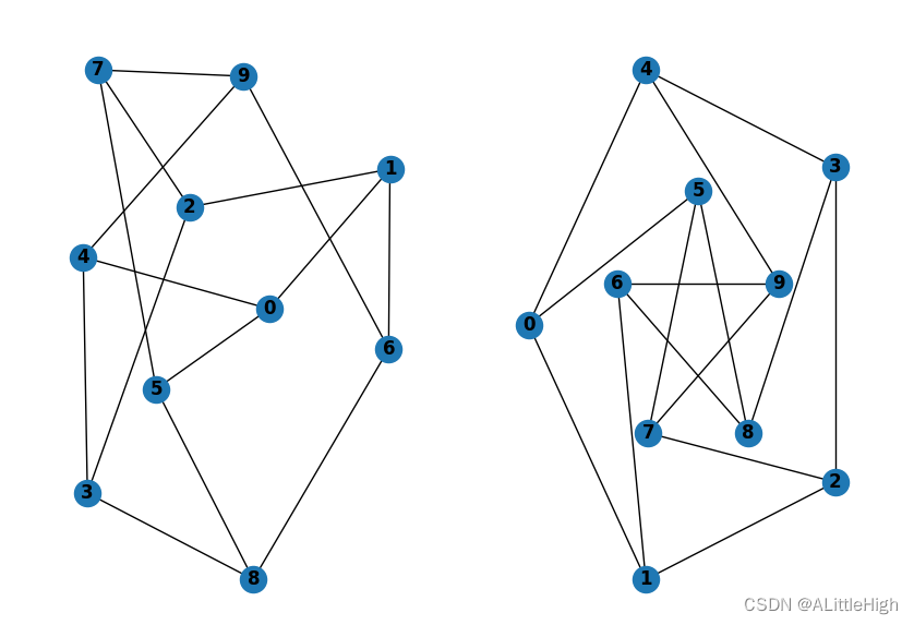
测试一下是否能正确绘图

import networkx as nx
import matplotlib.pyplot as plt

G = nx.petersen_graph()
subax1 = plt.subplot(121)
nx.draw(G, with_labels=True, font_weight='bold')
subax2 = plt.subplot(122)
nx.draw_shell(G, nlist=[range(5, 10), range(5)], with_labels=True, font_weight='bold')

plt.show()

在这里插入图片描述
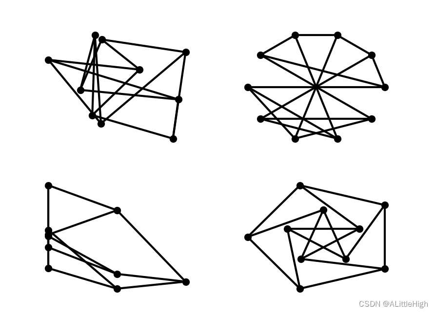
看一下其他的绘图方法

import networkx as nx
import matplotlib.pyplot as plt

G = nx.petersen_graph()
options = {
    
    
    'node_color': 'black',
    'node_size': 100,
    'width': 3,
}
subax1 = plt.subplot(221)
nx.draw_random(G, **options)
subax2 = plt.subplot(222)
nx.draw_circular(G, **options)
subax3 = plt.subplot(223)
nx.draw_spectral(G, **options)
subax4 = plt.subplot(224)
nx.draw_shell(G, nlist=[range(5, 10), range(5)], **options)
plt.show()

在这里插入图片描述
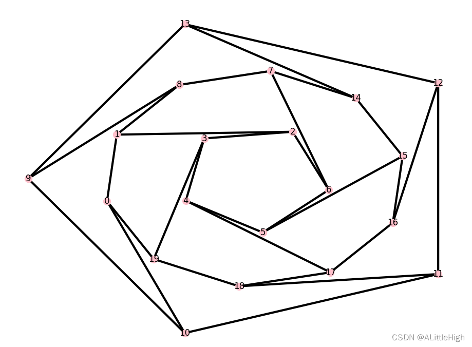
您可以通过draw_networkx()找到其他选项，并通过layout模块找到布局。您可以使用draw_shell()使用多个shell。

import networkx as nx
import matplotlib.pyplot as plt

G = nx.dodecahedral_graph()
shells = [[2, 3, 4, 5, 6], [8, 1, 0, 19, 18, 17, 16, 15, 14, 7], [9, 10, 11, 12, 13]]
options = {
    
    
    'node_color': 'pink',
    'node_size': 100,
    'width': 3,
}
nx.draw_shell(G, nlist=shells, **options, with_labels=True)
plt.show()

在这里插入图片描述

NX-Guides

在nx-guides中，可以了解到更多关于NetworkX，图像理论和网络分析的知识。在那里，你可以找到教程、实际应用以及对图和网络算法的深入研究。