1、Keras包和tensorflow包版本介绍
因为Keras包和tensorflow包的版本需要匹配才能使用,同时也要与python版本匹配才能使用。我目前的环境为 python3.5+keras2.1.0+tensorflow1.4.0。建议小白们如果不太懂各个版本该如何匹配的话,可以用我这个配套的包,我之前用python3.8,装上keras和tensorflow后,老是报错,实验了好几天才成功配置好环境的。然后注意千万不要在这个环境中安装gdal包了,装上gdal包后又会报错,原因貌似是gdal包把numpy版给降级了,导致keras和tensorflow报错。这是我的经验,可以参考一下。
2、损失函数(losses)介绍
损失函数文件(losses.py)在keras包我文件夹中可以找到(我的是在“D:\Anaconda3\setup\envs\py35_tf1.4.0_keras2.1.0\Lib\site-packages\keras”)。里面总共有
2.1、mean_squared_error函数
源码为:
def mean_squared_error(y_true, y_pred):
    return K.mean(K.square(y_pred - y_true), axis=-1)
公式为:
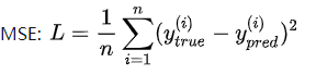
我们来举一个例子看看怎么来计算的。
假设:
y_true = [[0., 1., 1.], [0., 0., 1.]] ##真实标签
y_pred = [[1., 1., 0], [1., 0., 1]]  #预测标签,可见第一个列表里错了2个,第一个列表里错了1个
y_true = tf.convert_to_tensor(y_true) #将列表转成张量
y_pred = tf.convert_to_tensor(y_pred) #将列表转成张量,因为K.square和K.mean的输入类型为张量。
我们可以查看y_true和y_pred的类型,为张量:
type(y_true)
#tensorflow.python.framework.ops.Tensor
type(y_pred)
#tensorflow.python.framework.ops.Tensor
调用mean_squared_error函数计算:
def mean_squared_error(y_true, y_pred):
    return K.mean(K.square(y_pred - y_true),axis=-1)
result = mean_squared_error(y_true, y_pred)
type(result) #查看结果类型,也为张量
#tensorflow.python.framework.ops.Tensor
接下来查看result张量里的具体数值,这里要先调用tf.Session()。因为 上面的函数定义以及调用都只是先把计算所需要的内容准备好,搭了一个框架,并没有实际运算,Session 一下才能开始计算。下面的print结果为[0.6666667 0.33333334],说明第一个列表的损失为0.67,第二个为0.33。这个算法有点像计算方差。
with tf.Session() as sess:
    print (result.eval())
#[0.6666667  0.33333334]
2.2、mean_absolute_error函数
源码为:
def mean_absolute_error(y_true, y_pred):
    return K.mean(K.abs(y_pred - y_true), axis=-1)
公式为:
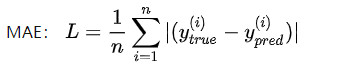
和上面的例子一样,运行方法一样。结果为[0.6666667 0.33333334],这个算法相当于计算平均绝对误差。
2.3、mean_absolute_percentage_error函数
源码为:
def mean_absolute_percentage_error(y_true, y_pred):
    diff = K.abs((y_true - y_pred) / K.clip(K.abs(y_true),K.epsilon(),None))
    return 100. * K.mean(diff, axis=-1)
公式为:
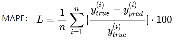
和上面的例子一样,运行方法一样。结果为[3.3333338e+08 3.3333331e+08],这个结果不是很懂有什么意义,但看公式像是预测错误占实际标签的百分比。
2.4、mean_squared_logarithmic_error函数
源码为:
def mean_squared_logarithmic_error(y_true, y_pred):
    first_log = K.log(K.clip(y_pred, K.epsilon(), None) + 1.)
    second_log = K.log(K.clip(y_true, K.epsilon(), None) + 1.)
    return K.mean(K.square(first_log - second_log), axis=-1)
公式为:
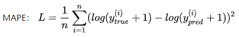
和上面的例子一样,运行方法一样。结果为[0.32030192 0.16015096]。
2.5、squared_hinge函数
源码为:
def squared_hinge(y_true, y_pred):
    return K.mean(K.square(K.maximum(1. - y_true * y_pred, 0.)), axis=-1)
公式为:
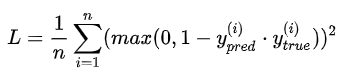
结果为[0.6666667 0.6666667]。由于只有0和1两个值,所以 y_true * y_pred相当于将正确预测的地方设为1,而错误预测的地方设为0,然后1. - y_true * y_pred则又将其反过来,得到错误预测的地方。
2.5、hinge函数
源码为:
def hinge(y_true, y_pred):
    return K.mean(K.maximum(1. - y_true * y_pred, 0.), axis=-1)
公式为:
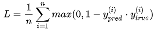
结果为[0.6666667 0.6666667]。
2.6、categorical_hinge函数
源码为:
def categorical_hinge(y_true, y_pred):
    pos = K.sum(y_true * y_pred, axis=-1)
    neg = K.max((1. - y_true) * y_pred, axis=-1)
    return K.maximum(0., neg - pos + 1.)
公式与hinge函数相同。pos表示将实际值为1的地方正确预测为1的个数,而neg则是将实际值为0的地方错误预测为1的个数。结果为[1. 1.]
2.7、logcosh函数
源码为:
def logcosh(y_true, y_pred):
    """Logarithm of the hyperbolic cosine of the prediction error.

    `log(cosh(x))` is approximately equal to `(x ** 2) / 2` for small `x` and
    to `abs(x) - log(2)` for large `x`. This means that 'logcosh' works mostly
    like the mean squared error, but will not be so strongly affected by the
    occasional wildly incorrect prediction. However, it may return NaNs if the
    intermediate value `cosh(y_pred - y_true)` is too large to be represented
    in the chosen precision.
    """
    def cosh(x):
        return (K.exp(x) + K.exp(-x)) / 2
    return K.mean(K.log(cosh(y_pred - y_true)), axis=-1)
预测误差的双曲余弦的对数。结果为[0.2891872 0.1445936]
2.8、categorical_crossentropy函数
源码为:
def categorical_crossentropy(y_true, y_pred):
    return K.categorical_crossentropy(y_true, y_pred)
更详细的源码见 .\Lib\site-packages\keras\backend\cntk_backend.py 中,如下:
def categorical_crossentropy(target, output, from_logits=False):
    if from_logits:
        result = C.cross_entropy_with_softmax(output, target)
        # cntk's result shape is (batch, 1), while keras expect (batch, )
        return C.reshape(result, ())
    else:
        # scale preds so that the class probas of each sample sum to 1
        output /= C.reduce_sum(output, axis=-1)
        # avoid numerical instability with epsilon clipping
        output = C.clip(output, epsilon(), 1.0 - epsilon())
        return -sum(target * C.log(output), axis=-1)
当使用categorical_crossentropy损失时,你的目标值应该是分类格式 (即,如果你有10个类,每个样本的目标值应该是一个10维的向量,这个向量除了表示类别的那个索引为1,其他均为0)。
2.9、sparse_categorical_crossentropy函数
源码为:
def sparse_categorical_crossentropy(target, output, from_logits=False):
    target = C.one_hot(target, output.shape[-1])
    target = C.reshape(target, output.shape)
    return categorical_crossentropy(target, output, from_logits)
意义与categorical_crossentropy相似。
2.10、binary_crossentropy函数
源码为:
def binary_crossentropy(target, output, from_logits=False):
    if from_logits:
        output = C.sigmoid(output)
    output = C.clip(output, epsilon(), 1.0 - epsilon())
    output = -target * C.log(output) - (1.0 - target) * C.log(1.0 - output)
    return output
二分类的交叉熵。
2.11、kullback_leibler_divergence函数
源码为:
def kullback_leibler_divergence(y_true, y_pred):
    y_true = K.clip(y_true, K.epsilon(), 1)
    y_pred = K.clip(y_pred, K.epsilon(), 1)
    return K.sum(y_true * K.log(y_true / y_pred), axis=-1)
KL散度计算损失
2.12、poisson函数
源码为:
def poisson(y_true, y_pred):
    return K.mean(y_pred - y_true * K.log(y_pred + K.epsilon()), axis=-1)
泊松损失函数
2.13、cosine_proximity函数
源码为:
def cosine_proximity(y_true, y_pred):
    y_true = K.l2_normalize(y_true, axis=-1)
    y_pred = K.l2_normalize(y_pred, axis=-1)
    return -K.sum(y_true * y_pred, axis=-1)
2.14、cosine_proximity函数
源码为:
def cosine_proximity(y_true, y_pred):
    y_true = K.l2_normalize(y_true, axis=-1)
    y_pred = K.l2_normalize(y_pred, axis=-1)
    return -K.sum(y_true * y_pred, axis=-1)