TensorFlow搭建VGG16训练CIFAR10数据集

本篇教程基于TensorFlow 2.5，使用VGG16网络训练CIFAR10数据集，模型最终在测试集上的准确率超过91%。

请注意，如果想使用GPU进行训练，需要确保TensorFlow版本和CUDA版本对应。可用以下指令检查是否成功调用GPU，若返回False，则说明不能调用GPU：

import tensorflow as tf

tf.test.is_gpu_available()

1、构建数据集

CIFAR10数据集是一个用于识别普适物体的小型数据集，一共包含10个类别的RGB三通道彩色图片，图片尺寸大小为32x32，如图所示：

在使用 TensorFlow 时，我们可以直接使用 tensorflow.keras.datasets.cifar10.load_data()方法获取该数据集。 

def load_images():
    (x_img_train, y_label_train), (x_img_test, y_label_test) = cifar10.load_data()

    x_img_train = x_img_train.astype(np.float32)  # 数据类型转换
    x_img_test = x_img_test.astype(np.float32)

    (x_img_train, x_img_test) = normalization(x_img_train, x_img_test)

    y_label_train = to_categorical(y_label_train, 10)  # one-hot
    y_label_test = to_categorical(y_label_test, 10)

    return x_img_train, y_label_train, x_img_test, y_label_test

2、数据增强

为了提高模型的泛化性，防止训练时在训练集上过拟合，往往在训练的过程中会对训练集进行数据增强操作，例如归一化、随机翻转、遮挡等操作。我们这里对训练集做如下处理：

    datagen = ImageDataGenerator(
        featurewise_center=False,  # 布尔值。将输入数据的均值设置为 0，逐特征进行。
        samplewise_center=False,  # 布尔值。将每个样本的均值设置为 0。
        featurewise_std_normalization=False,  # 布尔值。将输入除以数据标准差，逐特征进行。
        samplewise_std_normalization=False,  # 布尔值。将每个输入除以其标准差。
        zca_whitening=False,  # 布尔值。是否应用 ZCA 白化。
        rotation_range=15,  # 整数。随机旋转的度数范围 (degrees, 0 to 180)
        width_shift_range=0.1,  # randomly shift images horizontally (fraction of total width)
        height_shift_range=0.1,  # randomly shift images vertically (fraction of total height)
        horizontal_flip=True,  # 布尔值。随机水平翻转。
        vertical_flip=False)  # 布尔值。随机垂直翻转。

3、模型搭建

VGG是由Simonyan 和Zisserman在文献《Very Deep Convolutional Networks for Large Scale Image Recognition》中提出卷积神经网络模型，其名称来源于作者所在的牛津大学视觉几何组(Visual Geometry Group)的缩写。

该模型参加2014年的 ImageNet图像分类与定位挑战赛，取得了优异成绩：在分类任务上排名第二，在定位任务上排名第一。

VGG中根据卷积核大小和卷积层数目的不同，可分为 A，A-LRN,B,C,D,E 共6个配置(ConvNet Configuration)，其中以 D,E 两种配置较为常用，分别称为VGG16和VGG19。

下图给出了VGG的六种结构配置：

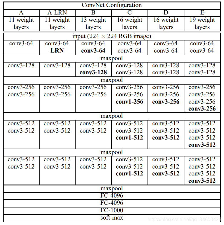
针对VGG16进行具体分析可以发现，VGG16共包含：

• 13个卷积层（Convolutional Layer），分别用conv3-XXX表示 
• 3个全连接层（Fully connected Layer）,分别用FC-XXXX表示 
• 5个池化层（Pool layer）,分别用maxpool表示 

其中，卷积层和全连接层具有权重系数，因此也被称为权重层，总数目为13+3=16，这即是VGG16中16的来源。(池化层不涉及权重，因此不属于权重层，不被计数)。

特点 

VGG16的突出特点是简单，体现在：

        1.卷积层均采用相同的卷积核参数

        卷积层均表示为conv3-XXX，其中conv3说明该卷积层采用的卷积核的尺寸(kernel size)是3，即宽（width）和高（height）均为3，3*3是很小的卷积核尺寸，结合其它参数（步幅stride=1，填充方式padding=same），这样就能够使得每一个卷积层(张量)与前一层（张量）保持相同的宽和高。XXX代表卷积层的通道数。

        2.池化层均采用相同的池化核参数

        池化层的参数均为2×。

        3.模型是由若干卷积层和池化层堆叠（stack）的方式构成，比较容易形成较深的网络结构（在2014年，16层已经被认为很深了）。

综合上述分析，可以概括VGG的优点为: Small filters, Deeper networks。

代码实现如下：

class ConvBNRelu(tf.keras.Model):
    def __init__(self, filters, kernel_size=3, strides=1, padding='SAME', weight_decay=0.0005, rate=0.4, drop=True):
        super(ConvBNRelu, self).__init__()
        self.drop = drop
        self.conv = keras.layers.Conv2D(filters=filters, kernel_size=kernel_size, strides=strides,
                                        padding=padding, kernel_regularizer=tf.keras.regularizers.l2(weight_decay))
        self.batchnorm = tf.keras.layers.BatchNormalization()
        self.dropOut = keras.layers.Dropout(rate=rate)

    def call(self, inputs):  # , training=False
        layer = self.conv(inputs)
        layer = tf.nn.relu(layer)
        layer = self.batchnorm(layer)

        # 用来控制conv是否有dropout层，对应类ConvBNRelu中的self.drop属性
        if self.drop:
            layer = self.dropOut(layer)

        return layer


class VGG16Model(tf.keras.Model):
    def __init__(self):
        super(VGG16Model, self).__init__()
        self.conv1 = ConvBNRelu(filters=64, kernel_size=[3, 3], rate=0.3)
        self.conv2 = ConvBNRelu(filters=64, kernel_size=[3, 3], drop=False)
        self.maxPooling1 = keras.layers.MaxPooling2D(pool_size=(2, 2))
        self.conv3 = ConvBNRelu(filters=128, kernel_size=[3, 3])
        self.conv4 = ConvBNRelu(filters=128, kernel_size=[3, 3], drop=False)
        self.maxPooling2 = keras.layers.MaxPooling2D(pool_size=(2, 2))
        self.conv5 = ConvBNRelu(filters=256, kernel_size=[3, 3])
        self.conv6 = ConvBNRelu(filters=256, kernel_size=[3, 3])
        self.conv7 = ConvBNRelu(filters=256, kernel_size=[3, 3], drop=False)
        self.maxPooling3 = keras.layers.MaxPooling2D(pool_size=(2, 2))
        self.conv11 = ConvBNRelu(filters=512, kernel_size=[3, 3])
        self.conv12 = ConvBNRelu(filters=512, kernel_size=[3, 3])
        self.conv13 = ConvBNRelu(filters=512, kernel_size=[3, 3], drop=False)
        self.maxPooling5 = keras.layers.MaxPooling2D(pool_size=(2, 2))
        self.conv14 = ConvBNRelu(filters=512, kernel_size=[3, 3])
        self.conv15 = ConvBNRelu(filters=512, kernel_size=[3, 3])
        self.conv16 = ConvBNRelu(filters=512, kernel_size=[3, 3], drop=False)
        self.maxPooling6 = keras.layers.MaxPooling2D(pool_size=(2, 2))
        self.flat = keras.layers.Flatten()
        self.dropOut = keras.layers.Dropout(rate=0.5)

        self.dense1 = keras.layers.Dense(units=512,
                                         activation='relu', kernel_regularizer=tf.keras.regularizers.l2(0.0005))
        self.batchnorm = tf.keras.layers.BatchNormalization()
        self.dense2 = keras.layers.Dense(units=10)
        self.softmax = keras.layers.Activation('softmax')

    def call(self, inputs):  # , training=False
        net = self.conv1(inputs)
        net = self.conv2(net)
        net = self.maxPooling1(net)
        net = self.conv3(net)
        net = self.conv4(net)
        net = self.maxPooling2(net)
        net = self.conv5(net)
        net = self.conv6(net)
        net = self.conv7(net)
        net = self.maxPooling3(net)
        net = self.conv11(net)
        net = self.conv12(net)
        net = self.conv13(net)
        net = self.maxPooling5(net)
        net = self.conv14(net)
        net = self.conv15(net)
        net = self.conv16(net)
        net = self.maxPooling6(net)
        net = self.dropOut(net)
        net = self.flat(net)
        net = self.dense1(net)
        net = self.batchnorm(net)
        net = self.dropOut(net)
        net = self.dense2(net)
        net = self.softmax(net)
        return net

4、训练策略

在模型的训练上，我们采用的策略是：batch_size大小为256，初始学习率为0.1，每经过20个epoch学习率变为原来的0.5，共训练100个epoch，损失函数采用交叉熵，优化器为SGD。

    # 超参数
    training_epochs = 100
    batch_size = 256
    learning_rate = 0.1
    momentum = 0.9  # SGD加速动量
    weight_decay = 1e-6  # 权重衰减
    lr_drop = 20  # 衰减倍数


    def lr_scheduler(epoch):  # 动态学习率衰减，epoch越大，lr衰减越剧烈。
        return learning_rate * (0.5 ** (epoch // lr_drop))


    reduce_lr = keras.callbacks.LearningRateScheduler(lr_scheduler)


    optimizer = tf.keras.optimizers.SGD(learning_rate=learning_rate,
                                        decay=weight_decay, momentum=momentum, nesterov=True)

    # 交叉熵、优化器，评价标准。
    model.compile(loss='categorical_crossentropy', optimizer=optimizer, metrics=['accuracy'])

5、结果可视化

可以借助 matplotlib 库绘制 accuracy 和 loss 曲线，以帮助我们分析训练过程，代码示例如下：

    from matplotlib import pyplot as plt
    
    plt.subplot(1, 2, 1)
    plt.plot(accuracy, label='Training Accuracy')
    plt.plot(val_accuracy, label='Validation Accuracy')
    plt.title('Training and Validation Accuracy')
    plt.legend()

    plt.subplot(1, 2, 2)
    plt.plot(loss, label='Training Loss')
    plt.plot(val_loss, label='Validation Loss')
    plt.title('Training and Validation Loss')
    plt.legend()

    plt.savefig('./results.png')
    plt.show()

6、完整代码

import numpy as np
import time
from matplotlib import pyplot as plt

import tensorflow as tf

# 调用显卡内存分配指令需要的包
from tensorflow.compat.v1 import ConfigProto
from tensorflow.compat.v1 import InteractiveSession

from tensorflow import keras
from tensorflow.keras.utils import to_categorical
from tensorflow.keras.datasets import cifar10
from tensorflow.keras.preprocessing.image import ImageDataGenerator

# 显卡内存分配指令：按需分配
config = ConfigProto()
config.gpu_options.allow_growth = True
session = InteractiveSession(config=config)


def normalization(x_img_train, x_img_test):
    mean = np.mean(x_img_train, axis=(0, 1, 2, 3))  # 四个维度 批数 像素x像素 通道数
    std = np.std(x_img_train, axis=(0, 1, 2, 3))
    # 测试集做一致的标准化 用到的均值和标准差 服从train的分布（有信息杂糅的可能）
    x_img_train = (x_img_train - mean) / (std + 1e-7)  # trick 加小数点 避免出现整数
    x_img_test = (x_img_test - mean) / (std + 1e-7)

    return x_img_train, x_img_test


# 数据读取
def load_images():
    (x_img_train, y_label_train), (x_img_test, y_label_test) = cifar10.load_data()

    x_img_train = x_img_train.astype(np.float32)  # 数据类型转换
    x_img_test = x_img_test.astype(np.float32)

    (x_img_train, x_img_test) = normalization(x_img_train, x_img_test)

    y_label_train = to_categorical(y_label_train, 10)  # one-hot
    y_label_test = to_categorical(y_label_test, 10)

    return x_img_train, y_label_train, x_img_test, y_label_test


class ConvBNRelu(tf.keras.Model):
    def __init__(self, filters, kernel_size=3, strides=1, padding='SAME', weight_decay=0.0005, rate=0.4, drop=True):
        super(ConvBNRelu, self).__init__()
        self.drop = drop
        self.conv = keras.layers.Conv2D(filters=filters, kernel_size=kernel_size, strides=strides,
                                        padding=padding, kernel_regularizer=tf.keras.regularizers.l2(weight_decay))
        self.batchnorm = tf.keras.layers.BatchNormalization()
        self.dropOut = keras.layers.Dropout(rate=rate)

    def call(self, inputs):  # , training=False
        layer = self.conv(inputs)
        layer = tf.nn.relu(layer)
        layer = self.batchnorm(layer)

        # 用来控制conv是否有dropout层，对应类ConvBNRelu中的self.drop属性
        if self.drop:
            layer = self.dropOut(layer)

        return layer


class VGG16Model(tf.keras.Model):
    def __init__(self):
        super(VGG16Model, self).__init__()
        self.conv1 = ConvBNRelu(filters=64, kernel_size=[3, 3], rate=0.3)
        self.conv2 = ConvBNRelu(filters=64, kernel_size=[3, 3], drop=False)
        self.maxPooling1 = keras.layers.MaxPooling2D(pool_size=(2, 2))
        self.conv3 = ConvBNRelu(filters=128, kernel_size=[3, 3])
        self.conv4 = ConvBNRelu(filters=128, kernel_size=[3, 3], drop=False)
        self.maxPooling2 = keras.layers.MaxPooling2D(pool_size=(2, 2))
        self.conv5 = ConvBNRelu(filters=256, kernel_size=[3, 3])
        self.conv6 = ConvBNRelu(filters=256, kernel_size=[3, 3])
        self.conv7 = ConvBNRelu(filters=256, kernel_size=[3, 3], drop=False)
        self.maxPooling3 = keras.layers.MaxPooling2D(pool_size=(2, 2))
        self.conv11 = ConvBNRelu(filters=512, kernel_size=[3, 3])
        self.conv12 = ConvBNRelu(filters=512, kernel_size=[3, 3])
        self.conv13 = ConvBNRelu(filters=512, kernel_size=[3, 3], drop=False)
        self.maxPooling5 = keras.layers.MaxPooling2D(pool_size=(2, 2))
        self.conv14 = ConvBNRelu(filters=512, kernel_size=[3, 3])
        self.conv15 = ConvBNRelu(filters=512, kernel_size=[3, 3])
        self.conv16 = ConvBNRelu(filters=512, kernel_size=[3, 3], drop=False)
        self.maxPooling6 = keras.layers.MaxPooling2D(pool_size=(2, 2))
        self.flat = keras.layers.Flatten()
        self.dropOut = keras.layers.Dropout(rate=0.5)

        self.dense1 = keras.layers.Dense(units=512,
                                         activation='relu', kernel_regularizer=tf.keras.regularizers.l2(0.0005))
        self.batchnorm = tf.keras.layers.BatchNormalization()
        self.dense2 = keras.layers.Dense(units=10)
        self.softmax = keras.layers.Activation('softmax')

    def call(self, inputs):  # , training=False
        net = self.conv1(inputs)
        net = self.conv2(net)
        net = self.maxPooling1(net)
        net = self.conv3(net)
        net = self.conv4(net)
        net = self.maxPooling2(net)
        net = self.conv5(net)
        net = self.conv6(net)
        net = self.conv7(net)
        net = self.maxPooling3(net)
        net = self.conv11(net)
        net = self.conv12(net)
        net = self.conv13(net)
        net = self.maxPooling5(net)
        net = self.conv14(net)
        net = self.conv15(net)
        net = self.conv16(net)
        net = self.maxPooling6(net)
        net = self.dropOut(net)
        net = self.flat(net)
        net = self.dense1(net)
        net = self.batchnorm(net)
        net = self.dropOut(net)
        net = self.dense2(net)
        net = self.softmax(net)
        return net


# 准备训练
if __name__ == '__main__':
    print('tf.__version__:', tf.__version__)
    print('keras.__version__:', keras.__version__)

    # 超参数
    training_epochs = 100
    batch_size = 256
    learning_rate = 0.1
    momentum = 0.9  # SGD加速动量
    weight_decay = 1e-6  # 权重衰减
    lr_drop = 20  # 衰减倍数

    tf.random.set_seed(2022)  # 固定随机种子，可复现


    def lr_scheduler(epoch):  # 动态学习率衰减，epoch越大，lr衰减越剧烈。
        return learning_rate * (0.5 ** (epoch // lr_drop))


    reduce_lr = keras.callbacks.LearningRateScheduler(lr_scheduler)

    x_img_train, y_label_train, x_img_test, y_label_test = load_images()

    datagen = ImageDataGenerator(
        featurewise_center=False,  # 布尔值。将输入数据的均值设置为 0，逐特征进行。
        samplewise_center=False,  # 布尔值。将每个样本的均值设置为 0。
        featurewise_std_normalization=False,  # 布尔值。将输入除以数据标准差，逐特征进行。
        samplewise_std_normalization=False,  # 布尔值。将每个输入除以其标准差。
        zca_whitening=False,  # 布尔值。是否应用 ZCA 白化。
        rotation_range=15,  # 整数。随机旋转的度数范围 (degrees, 0 to 180)
        width_shift_range=0.1,  # randomly shift images horizontally (fraction of total width)
        height_shift_range=0.1,  # randomly shift images vertically (fraction of total height)
        horizontal_flip=True,  # 布尔值。随机水平翻转。
        vertical_flip=False)  # 布尔值。随机垂直翻转。

    datagen.fit(x_img_train)

    model = VGG16Model()  # 调用模型

    optimizer = tf.keras.optimizers.SGD(learning_rate=learning_rate,
                                        decay=weight_decay, momentum=momentum, nesterov=True)
    # 交叉熵、优化器，评价标准。
    model.compile(loss='categorical_crossentropy', optimizer=optimizer, metrics=['accuracy'])

    t1 = time.time()
    history = model.fit(datagen.flow(x_img_train, y_label_train,
                                     batch_size=batch_size), epochs=training_epochs, verbose=2, callbacks=[reduce_lr],
                        steps_per_epoch=x_img_train.shape[0] // batch_size, validation_data=(x_img_test, y_label_test))
    t2 = time.time()
    CNNfit = float(t2 - t1)
    print("Time taken: {} seconds".format(CNNfit))

    accuracy = history.history['accuracy']
    val_accuracy = history.history['val_accuracy']
    loss = history.history['loss']
    val_loss = history.history['val_loss']

    plt.subplot(1, 2, 1)
    plt.plot(accuracy, label='Training Accuracy')
    plt.plot(val_accuracy, label='Validation Accuracy')
    plt.title('Training and Validation Accuracy')
    plt.legend()

    plt.subplot(1, 2, 2)
    plt.plot(loss, label='Training Loss')
    plt.plot(val_loss, label='Validation Loss')
    plt.title('Training and Validation Loss')
    plt.legend()

    plt.savefig('./results.png')
    plt.show()