CIFAR10数据集训练与测试

1.数据集介绍

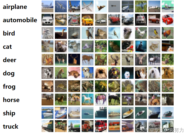
包含60000张32*32的彩色图片，它们共分为10类，其中50000张是训练图片，10000张是测试图片。

2.模型设计

在设计模型时，重点要关注的三个参数：
1.输入图片的通道数和尺寸
2.在连接到全连接层前的图片的通道数和尺寸
3.输出的分类数
诸：1和3主要由数据集决定，而2则是有模型的结构决定，需要计算。通道数一般卷积一次就会加倍，而图片尺寸一般逐渐随着卷积核池化逐渐减小，计算公式如下：

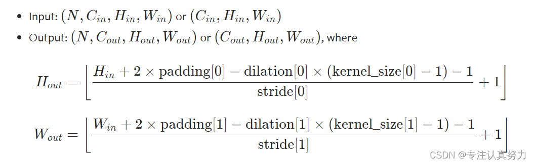
对于2的计算，如果模型很复杂，尤其网络特别深，我们要按照输入尺寸，从头到尾进行计算，这样太麻烦了。我们可以设计一个函数来求。
以下是我们设计的模型，现在要知道在经过多次卷积和池化后全连接层的输入元素有多少个？

class Net_CIFAR10(nn.Module):
    def __init__(self, in_channels=3, num_classes=10):
        super(Net_CIFAR10, self).__init__()
        self.layer1 = nn.Sequential(
            nn.Conv2d(in_channels, 32, 5),
            nn.ReLU(),
            nn.BatchNorm2d(32),

            nn.Conv2d(32, 32, 5),
            nn.ReLU(),
            nn.BatchNorm2d(32),

            nn.MaxPool2d(2, 2),

        )
        self.layer2 = nn.Sequential(
            nn.Conv2d(32, 64, 3),
            nn.ReLU(),
            nn.BatchNorm2d(64),

            nn.Conv2d(64, 64, 3),
            nn.ReLU(),
            nn.BatchNorm2d(64),

            nn.MaxPool2d(2, 2),

            nn.Conv2d(64, 128, 3),
            nn.ReLU(),
            nn.BatchNorm2d(128),
        )

我们首先根据数据集，设置一个batch = 64，具有3个通道的 32*32 的随机值张量，模拟我们的图片的输入。

model = MODELS.Net_CIFAR10()
inputs = Variable(torch.randn([64, 3, 32, 32]))
out = model.layer2(model.layer1(inputs))
print(inputs.size())
print(out.size())

输出结果

torch.Size([64, 3, 32, 32])
torch.Size([64, 128, 2, 2])

由此可知，我们可以将它展平为64个具有 128*2*2=512 个元素的一维张量，然后进行全连接输出10个分类。
即全连接层可以这样设置参数：

 self.fc = nn.Sequential(
            nn.Flatten(),
            nn.Linear(128 * 2 * 2, 128),
            nn.ReLU(),
            nn.Linear(128, num_classes)
        )

设计函数如下，注意不同的模型有不同的特征提取过程，需要修改函数中的第二行代码。

# 根据模型和输入图片的[C,W,H]得出全连接层的输入个数
def auto_fc_in(model, CWH):
    inputs = Variable(torch.randn([2] + CWH)) # 2为通道数，可以为大于1的任意值
    out = model.layer2(model.layer1(inputs))  # 注意不同的模型具有不同表达，可以概括为特征提取层
    C_out = out.size()[1]
    H_out = out.size()[2]
    W_out = out.size()[3]
    print('Number of input nodes at FC: %d*%d*%d=%d' % (C_out, H_out, W_out, C_out * H_out * W_out))

auto_fc_in(MODELS.Net_CIFAR10(), [3, 32, 32])

输出结果：

Number of input nodes at FC: 128*2*2=512

输出的 C*W*H=全连接层输入节点数

3.训练与测试

训练 100 轮，结果如下：

[95]: 81.73 %
[96]: 81.48 %
[97]: 81.88 %
[98]: 82.29 %
[99]: 80.99 %
Save model state in 82.55%
[100]: 82.55 %
Number of parameter: 0.22M
Max accuracy: 82.55 %
Average accuracy: 81.66 %
Average time per epoch:6.73 s

4.模型设计的相关改进

1. BN 和 dropout 一般不同时使用，如果一定要同时使用，可以将 dropout 放置于 BN 后面。
2. -> CONV/FC -> BatchNorm -> ReLu(or other activation) -> Dropout -> CONV/FC ->
   无论是理论上的分析，还是现代深度模型的演变，或者是实验的结果，BN 技术已显示出其优于 Dropout 的正则化效果。
3. Dropout 过时了，能发挥其作用的地方在全连接层，可当代的深度网络中，全连接层也在慢慢被全局平均池化曾所取代，不但能减低模型尺寸，还可以提升性能。
4. 池化层一般夹在卷积层的中间。

5.全连接层的两种选择

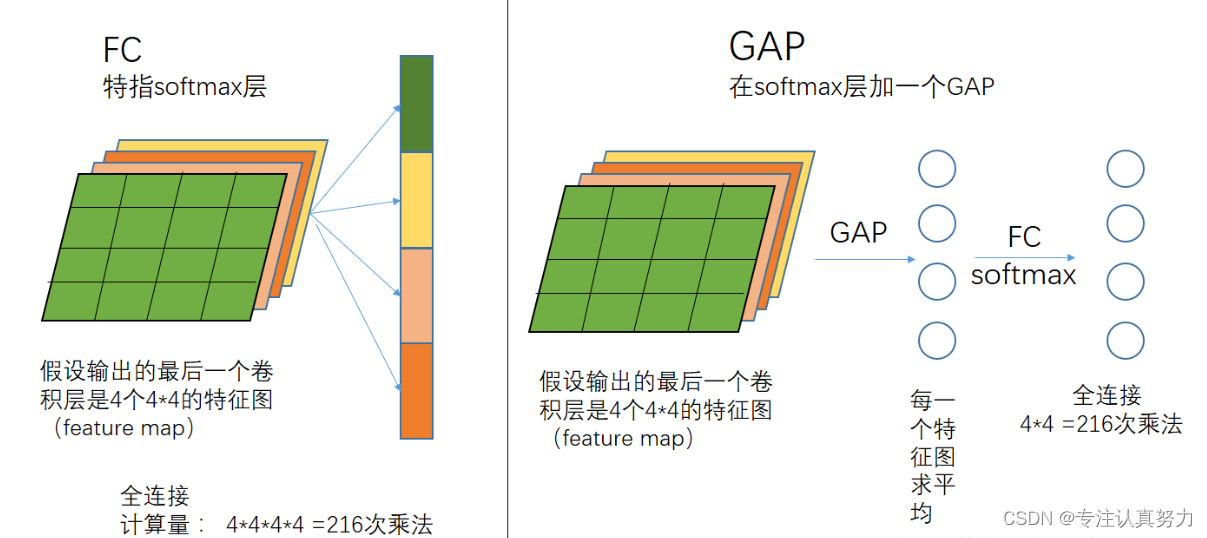
1.FC

self.fc = nn.Sequential(
            nn.Flatten(),
            nn.Linear(128 * 1 * 1, 64),
            nn.ReLU(),
            nn.Linear(64, num_classes)
        )

优点：可保持较大的模型capacity从而保证模型表示能力的迁移。
缺点：参数多，容易过拟合，对输入特征图的尺寸有要求，需要计算。

2.GAP

self.fc = nn.Sequential(
            nn.AdaptiveAvgPool2d((1,1)),
            nn.Flatten(),
            nn.Linear(128,num_classes)
        )

对整个网路在结构上做正则化防止过拟合。其直接剔除了全连接层中黑箱的特征，直接赋予了每个channel实际的类别意义。做法是在最后卷积层输出多少类别就多少map，然后直接分别对map进行平均值计算得到结果最后用softmax进行分类。
优点：克服了FC的缺点。不需要计算全连接池的输入尺寸了，128个特征图变为128个平均值了，然后连接输出为10个类别。
缺点：收敛速度慢。

GAP 对于我们设计模型的意义在于：可以只关注图片的通道数变化了，一般是一次卷积加倍一次通道数，对于特征图尺寸只要保证其不小于模型的下采样倍数即可。

6.实验与改进

以前面的模型和参数作为 baseline，对其进行改进如下，目的是提高测试集准确度，减少泛化误差，模型参数量和运算量。

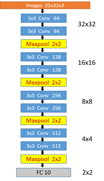
1. 八层卷积模型

模型结构

模型

class Net_CIFAR10_8Conv(nn.Module):
    def __init__(self, in_channels=3, num_classes=10):
        super(Net_CIFAR10_8Conv, self).__init__()
        self.layer1 = nn.Sequential(
            nn.Conv2d(in_channels, 64, 3, padding=1),
            nn.BatchNorm2d(64),

            nn.Conv2d(64, 64, 3, padding=1),
            nn.BatchNorm2d(64),
            nn.ReLU(inplace=True),

            nn.MaxPool2d(2, 2),
        )
        self.layer2 = nn.Sequential(
            nn.Conv2d(64, 128, 3, padding=1),
            nn.BatchNorm2d(128),

            nn.Conv2d(128, 128, 3, padding=1),
            nn.BatchNorm2d(128),
            nn.ReLU(inplace=True),

            nn.MaxPool2d(2, 2),
        )
        self.layer3 = nn.Sequential(
            nn.Conv2d(128, 256, 3, padding=1),
            nn.BatchNorm2d(256),

            nn.Conv2d(256, 256, 3, padding=1),
            nn.BatchNorm2d(256),
            nn.ReLU(inplace=True),

            nn.MaxPool2d(2, 2),
        )
        self.layer4 = nn.Sequential(
            nn.Conv2d(256, 512, 3, padding=1),
            nn.BatchNorm2d(512),

            nn.Conv2d(512, 512, 3, padding=1),
            nn.BatchNorm2d(512),
            nn.ReLU(inplace=True),

            nn.MaxPool2d(2, 2),
        )
        self.fc = nn.Sequential(
            nn.AdaptiveAvgPool2d((1, 1)),
            nn.Flatten(),
            nn.Dropout(0.4),
            nn.Linear(512, 256),
            nn.Linear(256, 64),
            nn.Linear(64, num_classes)
        )

    def forward(self, x):
        out = self.layer1(x)
        out = self.layer2(out)
        out = self.layer3(out)
        out = self.layer4(out)
        out = self.fc(out)
        return out

超参数

# hyper parameter
batch_size = 512
lr = 0.06
momentum = 0.9
total_epoch = 20
# configuration
device = torch.device('cuda' if torch.cuda.is_available() else 'cpu')
num_workers = 5
dataset_path = './data'
# Prepare dataset
train_loader, test_loader = CNN_FUN.CIFAR10_LOAD(dataset_path, batch_size, num_workers)
# Design model
# model = torchvision.models.DenseNet().to(device)
model = MODELS.Net_CIFAR10_8Conv().to(device)
# Construct loss and optimizer
criterion = nn.CrossEntropyLoss()
optimizer = torch.optim.SGD(model.parameters(), lr=lr, momentum=momentum, weight_decay=5e-3)
scheduler = lr_scheduler.ReduceLROnPlateau(optimizer, mode='min', factor=0.9, patience=5, verbose=True,
                                           threshold=0.005, threshold_mode='rel', cooldown=100, min_lr=0, eps=1e-03)
# Train and test
CNN_FUN.Train_Test(model, train_loader, test_loader, total_epoch, criterion, optimizer, scheduler, device)

结果

Number of parameter: 4.84M
Max accuracy: 85.62 %
Average accuracy: 83.91 %
Average time per epoch:13.96 s

2. 残差结构替代二层卷积结构

[64, ‘M’, 128, ‘M’, 256, ‘M’, 512, ‘M’]

class Conv_Block(nn.Module):
    def __init__(self, inchannel, outchannel, res=True):
        super(Conv_Block, self).__init__()
        self.res = res  # 是否带残差连接
        self.left = nn.Sequential(
            nn.Conv2d(inchannel, outchannel, 3, padding=1, stride=1, bias=False),
            nn.BatchNorm2d(outchannel),
            nn.ReLU(inplace=True),
            nn.Conv2d(outchannel, outchannel, 3, padding=1, stride=1, bias=False),
            nn.BatchNorm2d(outchannel),
        )
        self.shortcut = nn.Sequential(
            nn.Conv2d(inchannel, outchannel, 1, bias=False),
            nn.BatchNorm2d(outchannel)
        )
        self.relu = nn.Sequential(
            nn.ReLU(inplace=True)
        )

    def forward(self, x):
        out = self.left(x)
        if self.res:
            out += self.shortcut(x)
        out = self.relu(out)
        return out

class Res_Model(nn.Module):
    def __init__(self, res=True, inchannel=3, outchannel=10):
        super(Res_Model, self).__init__()

        self.block1 = Conv_Block(inchannel, 64)
        self.block2 = Conv_Block(64, 128)
        self.block3 = Conv_Block(128, 256)
        self.block4 = Conv_Block(256, 512)
        self.classifier = nn.Sequential(
            nn.AdaptiveAvgPool2d((1, 1)),
            nn.Flatten(),
            nn.Dropout(0.4),
            nn.Linear(512, 256),
            nn.Linear(256, 64),
            nn.Linear(64, outchannel)
        )  # 9 全连接层 )   # fc，最终Cifar10输出是10类

        self.relu = nn.ReLU(inplace=True)
        self.maxpool = nn.MaxPool2d(kernel_size=2, stride=2)

    def forward(self, x):
        out = self.block1(x)  # 32*32
        out = self.maxpool(out)  # 16*16
        out = self.block2(out)  # 16*16
        out = self.maxpool(out)  # 8*8
        out = self.block3(out)  # 8*8
        out = self.maxpool(out)  # 4*4
        out = self.block4(out)  # 4*4
        out = self.maxpool(out)  # 2*2
        out = self.classifier(out)  # 1*1
        return out

结果

Number of parameter: 5.01M
Max accuracy: 82.05 %
Average accuracy: 78.05 %
Average time per epoch:15.64 s

3. 增加不改变通道数的残差层

[64, ‘M’, 128, 128, ‘M’, 256, 256, ‘M’, 512, 512,‘M’]

class Conv_Block(nn.Module):
    def __init__(self, inchannel, outchannel, res=True):
        super(Conv_Block, self).__init__()
        self.res = res  # 是否带残差连接
        self.left = nn.Sequential(
            nn.Conv2d(inchannel, outchannel, 3, padding=1, stride=1, bias=False),
            nn.BatchNorm2d(outchannel),
            nn.ReLU(inplace=True),
            nn.Conv2d(outchannel, outchannel, 3, padding=1, stride=1, bias=False),
            nn.BatchNorm2d(outchannel),
        )
        self.shortcut = nn.Sequential(
            nn.Conv2d(inchannel, outchannel, 1, bias=False),
            nn.BatchNorm2d(outchannel)
        )
        self.relu = nn.Sequential(
            nn.ReLU(inplace=True)
        )

    def forward(self, x):
        out = self.left(x)
        if self.res:
            out += self.shortcut(x)
        out = self.relu(out)
        return out

class Res_Model(nn.Module):
    def __init__(self, res=True, inchannel=3, outchannel=10):
        super(Res_Model, self).__init__()

        self.block1 = Conv_Block(inchannel, 64)
        self.block2 = Conv_Block(64, 128)
        self.block3 = Conv_Block(128, 128)
        self.block4 = Conv_Block(128, 256)
        self.block5 = Conv_Block(256, 256)
        self.block6 = Conv_Block(256, 512)
        self.block7 = Conv_Block(512, 512)
        self.classifier = nn.Sequential(
            nn.AdaptiveAvgPool2d((1, 1)),
            nn.Flatten(),
            nn.Dropout(0.4),
            nn.Linear(512, 256),
            nn.Linear(256, 64),
            nn.Linear(64, outchannel)
        )  # 9 全连接层 )   # fc，最终Cifar10输出是10类

        self.relu = nn.ReLU(inplace=True)
        self.maxpool = nn.MaxPool2d(kernel_size=2, stride=2)

    def forward(self, x):
        out = self.block1(x)  # 32*32
        out = self.maxpool(out)  # 16*16
        out = self.block2(out)  # 16*16
        out = self.block3(out)  # 16*16
        out = self.maxpool(out)  # 8*8
        out = self.block4(out)  # 8*8
        out = self.block5(out)  # 8*8
        out = self.maxpool(out)  # 4*4
        out = self.block6(out)  # 4*4
        out = self.block7(out)  # 4*4
        out = self.maxpool(out)  # 2*2
        out = self.classifier(out)  # 1*1
        return out

结果

Number of parameter: 11.55M
Max accuracy: 85.15 %
Average accuracy: 81.12 %
Average time per epoch:24.33 s

4. 使用改进残差块

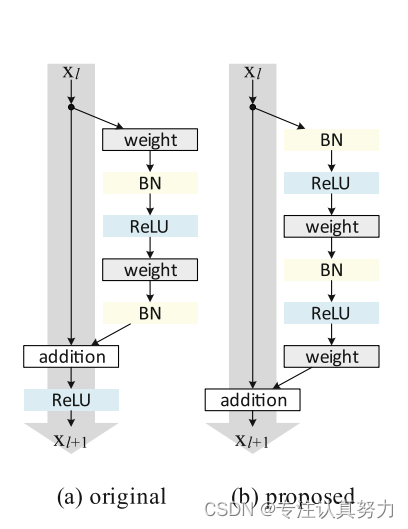
class Conv_Block(nn.Module):
    def __init__(self, inchannel, outchannel, res=True):
        super(Conv_Block, self).__init__()
        self.res = res  # 是否带残差连接
        self.left = nn.Sequential(
            nn.BatchNorm2d(inchannel),
            nn.ReLU(inplace=True),
            nn.Conv2d(inchannel, outchannel, 3, padding=1, stride=1, bias=False),
            nn.BatchNorm2d(outchannel),
            nn.ReLU(inplace=True),
            nn.Conv2d(outchannel, outchannel, 3, padding=1, stride=1, bias=False),
        )
        self.shortcut = nn.Sequential(
            nn.Conv2d(inchannel, outchannel, 1, bias=False),
            nn.BatchNorm2d(outchannel)
        )

    def forward(self, x):
        out = self.left(x)
        if self.res:
            out += self.shortcut(x)
        return out

self.classifier = nn.Sequential(
    nn.AdaptiveAvgPool2d((1, 1)),
    nn.Flatten(),
    nn.Linear(512, outchannel),
)

batch_size = 128
optimizer = torch.optim.SGD(model.parameters(), lr=lr, momentum=momentum, weight_decay=5e-4)
scheduler = lr_scheduler.CosineAnnealingLR(optimizer, T_max=total_epoch)

结果

Number of parameter: 11.49M
Max accuracy: 90.79 %
Average accuracy: 90.51 %
Average time per epoch:23.54 s

5.使用卷积替代全连接

batch_size = 64

self.classifier = nn.Sequential(
    Conv_Block(512, outchannel),
    nn.AdaptiveAvgPool2d((1, 1)),
    nn.Flatten()
)

结果

Number of parameter: 11.53M
Max accuracy: 92.63 %
Average accuracy: 92.35 %
Average time per epoch:28.22 s		

6.其他改进

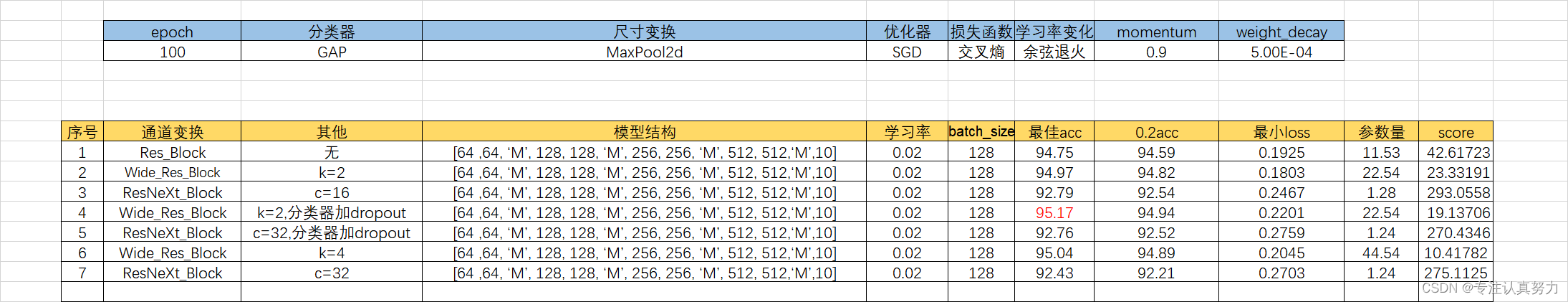
设置随机参数种子，保证实验结果可复现。

def seed_torch(seed=3407):
    random.seed(seed)
    os.environ['PYTHONHASHSEED'] = str(seed)
    np.random.seed(seed)
    torch.manual_seed(seed)
    torch.cuda.manual_seed_all(seed)
    torch.backends.cudnn.benchmark = False
    torch.backends.cudnn.deterministic = True
    torch.backends.cudnn.enabled = False

params: 22.54M
max acc: 95.14 %
average acc: 94.88 %
eopch time:30.46 s

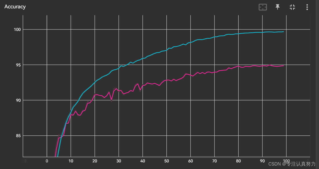
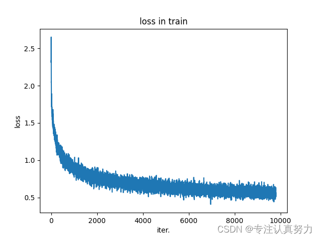
分析：泛化误差为训练精度和验证精度的差值，观察上图可知，随着训练的进行，泛化误差在增加