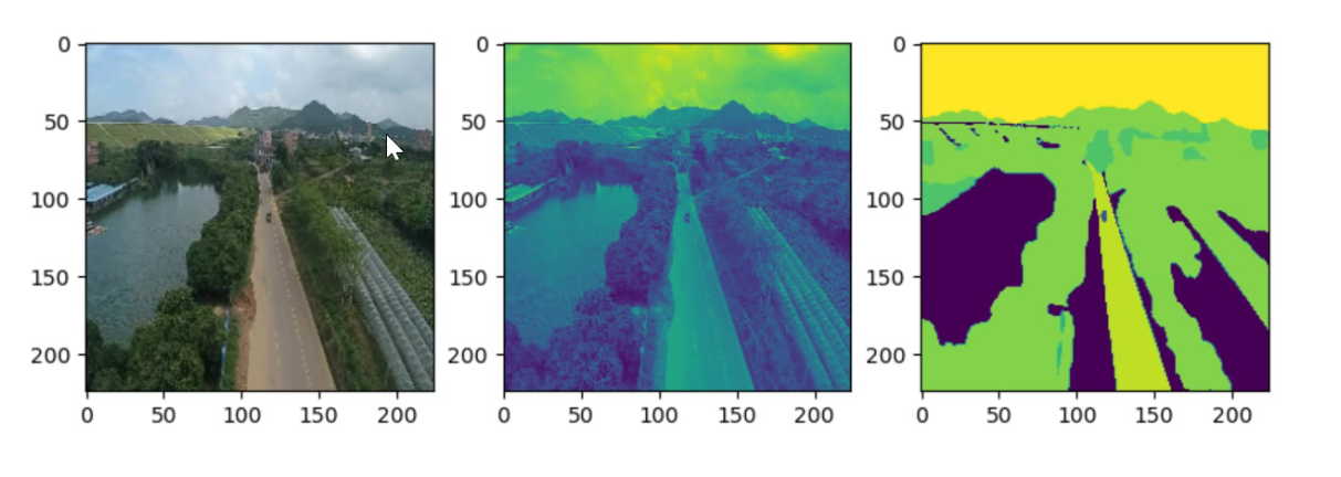
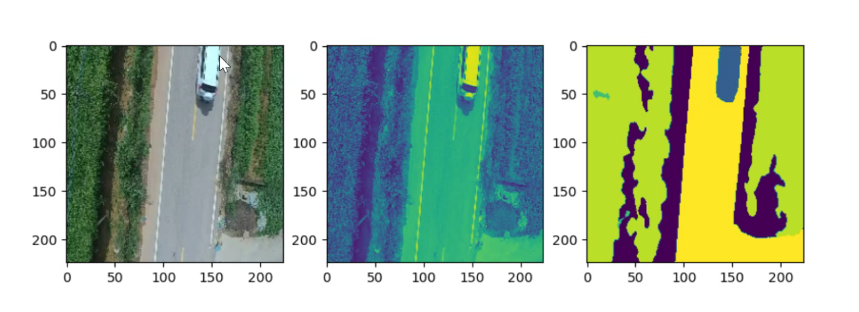
1.航拍图像分割效果展示:
2.背景介绍:
随着无人机技术的快速发展,无人机在研究领域和工业应用方面受到了广泛的关注.图像和视频是无人机感知周围环境的重要途径.图像语义分割是计算机视觉领域的研究热点,在无人驾驶,智能机器人等场景中应用广泛.无人机航拍图像语义分割是在无人机航拍图像的基础上,运用语义分割技术使无人机获得场景目标智能感知能力.介绍了语义分割技术和无人机的应用发展,相关无人机航拍数据集,无人机航拍图像特点和常用语义分割评价指标.针对无人机航拍的特点介绍了相关语义分割方法,包括小目标,模型实时性和多尺度整合等方面.综述无人机语义分割相关应用,包括线检测,农业和建筑物提取等方向,并分析无人机语义分割未来发展趋势和挑战.
3.数据增强
我们现在拥有的是大尺寸的航拍图像,我们不能直接把这些图像送入网络进行训练,因为内存承受不了而且他们的尺寸也各不相同。因此,我们首先将他们做随机切割,即随机生成x,y坐标,然后抠出该坐标下256*256的小图,并做以下数据增强操作:
1.原图和label图都需要旋转:90度,180度,270度
2.原图和label图都需要做沿y轴的镜像操作
3.原图做模糊操作
4.原图做光照调整操作
5.原图做增加噪声操作(高斯噪声,椒盐噪声)
这里我没有采用Keras自带的数据增广函数,而是自己使用opencv编写了相应的增强函数。
img_w = 256 img_h = 256 image_sets = ['1.png','2.png','3.png','4.png','5.png']defgamma_transform(img, gamma): gamma_table = [np.power(x / 255.0, gamma) * 255.0 forx inrange(256)] gamma_table = np.round(np.array(gamma_table)).astype(np.uint8) returncv2.LUT(img, gamma_table)defrandom_gamma_transform(img, gamma_vari): log_gamma_vari = np.log(gamma_vari) alpha = np.random.uniform(-log_gamma_vari, log_gamma_vari) gamma = np.exp(alpha) returngamma_transform(img, gamma) defrotate(xb,yb,angle): M_rotate = cv2.getRotationMatrix2D((img_w/2, img_h/2), angle, 1) xb = cv2.warpAffine(xb, M_rotate, (img_w, img_h)) yb = cv2.warpAffine(yb, M_rotate, (img_w, img_h)) returnxb,yb defblur(img): img = cv2.blur(img, (3, 3)); returnimgdefadd_noise(img): fori inrange(200): #添加点噪声temp_x = np.random.randint(0,img.shape[0]) temp_y = np.random.randint(0,img.shape[1]) img[temp_x][temp_y] = 255 returnimg defdata_augment(xb,yb): ifnp.random.random() < 0.25: xb,yb = rotate(xb,yb,90)

ifnp.random.random() < 0.25: xb,yb = rotate(xb,yb,180)

ifnp.random.random() < 0.25: xb,yb = rotate(xb,yb,270)

ifnp.random.random() < 0.25: xb = cv2.flip(xb, 1)

# flipcode > 0:沿y轴翻转yb = cv2.flip(yb, 1) ifnp.random.random() < 0.25: xb = random_gamma_transform(xb,1.0) ifnp.random.random() < 0.25: xb = blur(xb) ifnp.random.random() < 0.2: xb = add_noise(xb) returnxb,ybdefcreat_dataset(image_num = 100000, mode = 'original'): print('creating dataset...') image_each = image_num / len(image_sets) g_count = 0 fori intqdm(range(len(image_sets))): count = 0 src_img = cv2.imread('./data/src/'+ image_sets[i])

# 3 channelslabel_img = cv2.imread('./data/label/'+ image_sets[i],cv2.IMREAD_GRAYSCALE)

# single channelX_height,X_width,_ = src_img.shape

whilecount < image_each: random_width = random.randint(0, X_width - img_w - 1) random_height = random.randint(0, X_height - img_h - 1) src_roi = src_img[random_height: random_height + img_h, random_width: random_width + img_w,:] label_roi = label_img[random_height: random_height + img_h, random_width: random_width + img_w]

ifmode == 'augment': src_roi,label_roi = data_augment(src_roi,label_roi) visualize = np.zeros((256,256)).astype(np.uint8) visualize = label_roi *50 cv2.imwrite(('./aug/train/visualize/%d.png'% g_count),visualize) cv2.imwrite(('./aug/train/src/%d.png'% g_count),src_roi) cv2.imwrite(('./aug/train/label/%d.png'% g_count),label_roi) count += 1 g_count += 1
4.环境配置
tensorflow-gpu2.3.0
numpy1.21.5
matplotlib==3.5.1
5. 创建数据集路径索引文件
项目根目录下的"./prepare_dataset"目录下有三个文件:drive.py,stare.py和chasedb1.py。分别将三个文件中的“data_root_path”参数赋值为上述3.2准备好的数据集的绝对路径(例如: data_root_path=“/home/lee/datasets”)。然后分别运行:
python ./prepare_dataset/drive.py
python ./prepare_dataset/stare.py
python ./prepare_dataset/chasedb1.py
即可在"./prepare_dataset/data_path_list"目录下对应的数据集文件夹中生成"train.txt"和"test.txt"文件,分别存储了用于训练和测试的数据路径(每行依次存储原图,标签和FOV路径(用空格隔开))。
6.训练模型
在根目录下的"config.py"文件中修改超参数以及其他配置信息。特别要注意 “train_data_path_list"和"test_data_path_list"这两个参数,分别指向3.3中创建的某一个数据集的"train.txt"和"text.txt"。 在"train.py"中构造创建好的模型(所有模型都在"./models"内手撕),例如指定UNet模型:
net = models.UNetFamily.U_Net(1,2).to(device) # line 103 in train.py
修改完成后,在项目根目录执行:
CUDA_VISIBLE_DEVICES=1 python train.py --save UNet_vessel_seg --batch_size 64
上述命令将在1号GPU上执行训练程序,训练结果保存在“ ./experiments/UNet_vessel_seg”文件夹中,batchsize取64,其余参数取config.py中的默认参数。
可以在config中配置培训信息,也可以用命令行修改配置参数。训练结果将保存到“ ./experiments”文件夹中的相应目录(保存目录的名称用参数"–save"指定)。
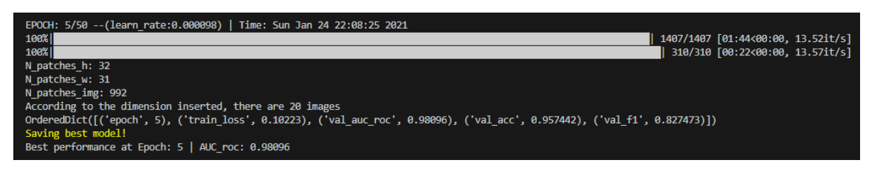
此外,需要注意一点,config文件中有个“val_on_test”参数。当其为真时表示会在训练的每个epoch结束后在测试集上进行性能评估,并选取"AUC of ROC"最高的模型保存为“best_model.pth”;当其为假时,会用验证集性能评估结果(AUC of ROC)保存模型。当然保存最佳模型依据的指标可以自行修改,默认为AUC of ROC。
7.测试评估
在“test.py”文件中构造对应的模型(同上),例如指定UNet模型:
net = models.UNetFamily.U_Net(1,2).to(device)
测试过程也需要"./config.py"中的相关参数,也可以在运行时通过命令行参数修改。
然后运行:
CUDA_VISIBLE_DEVICES=1 python test.py --save UNet_vessel_seg
上述命令将训练好的“./experiments /UNet_vessel_seg/best_model.pth”参数加载到相应的模型,并在测试集上进行性能测试,其测试性能指标结果保存在同一文件夹中的"performance.txt"中,同时会绘制相应的可视化结果。
8.系统整合:
9.完整源码&环境部署视频教程&数据集:
10.参考文献
[1]Hoover,A.,Kouznetsova,V.,Goldbaum,M.Locating blood vessels in retinal images by piecewise threshold probing of a matched filter response[].IEEE Trans Med Imag.2000
[2]Ying Sun.Automated identification of vessel contours in coronary arteriograms by an adaptive tracking algorithm[].IEEE Transactions on Microwave Theory and Techniques.1989
[3]Eckhorn R,Reitboeck H J,Arndt M,et al.Feature Linking via Synchronization among Distributed Assemblies:Simulation of Results from Cat Cortex[].Neural Computation.1990
[4]Chaudhuri S,Chatterjee S,Katz N,et al.Detection of bloodvessels in retinal images using two-dimensional matched filters[].IEEE Transactions on Medical Imaging.1989
[5]HOOVER A.Structured analysis of the retina. http://www.ces.clemson.edu/~ahoover/stare/ . 2000