DBNet模型

一、简述

DBNet是基于分割的文本检测算法，算法将可微分二值化模块(Differentiable Binarization)引入了分割模型，使得模型能够通过自适应的阈值图进行二值化，并且自适应阈值图可以计算损失，能够在模型训练过程中起到辅助效果优化的效果。经过验证，该方案不仅提升了文本检测的效果而且简化了后处理过程。相较于其他文本检测模型，DBNet在效果和性能上都有比较大的优势，是当前常用的文本检测算法。

二、模型结构

在这里插入图片描述 DB文本检测模型可以分为三个部分：

Backbone网络，负责提取图像的特征

FPN网络，特征金子塔，结构增强特征

Head网络，计算文本区域概率图

1.Backbone网络

DB文本检测网络的Backbone部分采用的是图像分类网络，论文中分别使用了ResNet50和ResNet18网络。这里结合具体的输入图像尺寸进行说明如下：
输入图像[1，3，640, 640] ，进入Backbone骨架网络，先经过一次卷积计算尺寸变为原来的1/2，而后经过四次下采样，输出四个尺度特征图如下：

在这里插入图片描述

2.FPN网络

特征金字塔结构FPN是一种卷积网络来高效提取图片中各维度特征的常用方法。
FPN网络的输入为Backbone部分的输出，经FPN计算后输出的特征图的高度和宽度为原图的1/4, 即[1, 256, 160, 160] 。
在这里插入图片描述

1/32特征图: [1, N, 20, 20] ===> 卷积 + 8倍上采样 ===> [1, 64, 160, 160]
1/16特征图：[1, N, 40, 40] ===> 加1/32特征图的两倍上采样 ===> 新1/16特征图 ==> 卷积 + 4倍上采样 ===> [1, 64, 160, 160]
1/8特征图：[1, N, 80, 80] ===> 加新1/16特征图的两倍上采样 ===>新1/8特征图 ===> 卷积 + 2倍上采样 ===> [1, 64, 160, 160]
1/4特征图：[1, N, 160, 160] ===> 加新1/8特征图的两倍上采样 ===> 新1/4特征图 ===> 卷积 ===> [1, 64, 160, 160]
融合特征图：[1, 256, 160, 160] # 将1/4，1/8, 1/16, 1/32特征图按通道层合并在一起

3.Head网络

计算文本区域概率图，文本区域阈值图以文本区域二值图。
Head网络会在FPN特征的基础上作上采样，将FPN特征由原来的1/4大小映射到原图大小，最终将生成的三个图合并，输出为[1, 3, 640, 640]
在这里插入图片描述

三、标签生成

DB算法在进行模型训练的时，需要根据标注框生成两幅图像：概率图和阈值图。生成过程如下图所示：
在这里插入图片描述
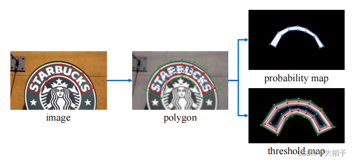
image图像中的红线是文本的标注框，文本标注框的点集合用如下形式表示：
$G = \{S_k\}_{k=1}^n$ , n表示顶点的数量
在polygon图像中，将红色的标注框外扩distance得到绿色的polygon框，内缩distance得到蓝色的polygon框。
论文中标注框内缩和外扩使用相同的distance,其计算公式为：
$=\cfrac{A(1 - r^2)}{L}$ , L代表周长，A代表面积，r代表缩放比例,通常r=0.4
多边形轮廓的周长L和面积A通过Polygon库计算获得。
根据计算出的distance，对标注框进行外扩和内缩操作，用Vatti算法实现，参考链接https://github.com/fonttools/pyclipper和中文文档https://www.cnblogs.com/zhigu/p/11943118.html，在python中调用pyclipper库的接口操作即可，简单示例如下。

import cv2
import pyclipper
import numpy as np
from shapely.geometry import Polygon

def draw_img(subject, canvas, color=(255,0,0)):
    """作图函数"""
    for i in range(len(subject)):
        j = (i+1)%len(subject)
        cv2.line(canvas, subject[i], subject[j], color)

# 论文默认shrink值
r=0.4
# 假定标注框
subject = ((100, 100), (250, 100), (250, 200), (100, 200))
# 创建Polygon对象
polygon = Polygon(subject)
# 计算偏置distance
distance = polygon.area*(1-np.power(r, 2))/polygon.length
print(distance)
# 25.2

# 创建PyclipperOffset对象
padding = pyclipper.PyclipperOffset()
# 向ClipperOffset对象添加一个路径用来准备偏置
# padding.AddPath(subject, pyclipper.JT_ROUND, pyclipper.ET_CLOSEDPOLYGON)
# adding.AddPath(subject, pyclipper.JT_SQUARE, pyclipper.ET_CLOSEDPOLYGON)
padding.AddPath(subject, pyclipper.JT_MITER, pyclipper.ET_CLOSEDPOLYGON)

# polygon外扩
polygon_expand = padding.Execute(distance)[0]
polygon_expand = [tuple(l) for l in polygon_expand]
print(polygon_expand)
# [(75, 75), (275, 75), (275, 225), (75, 225)]
# polygon内缩
polygon_shrink = padding.Execute(-distance)[0]
polygon_shrink = [tuple(l) for l in polygon_shrink]
print(polygon_shrink)
# [(125, 125), (225, 125), (225, 175), (125, 175)]

# 作图
canvas = np.zeros((300,350,3), dtype=np.uint8)
# 原轮廓用红色线条展示
draw_img(subject, canvas, color=(0,0,255))
# 外扩轮廓用绿色线条展示
draw_img(polygon_expand, canvas, color=(0,255,0))
# 内缩轮廓用蓝色线条展示
draw_img(polygon_shrink, canvas, color=(255,0,0))

cv2.imshow("Canvas", canvas) 
cv2.waitKey(0)

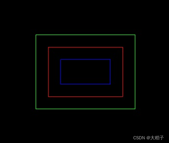
整体效果图如下，红色框为标注框，绿色框外扩后的效果，蓝色框为内缩后的效果。
在这里插入图片描述

0.示例说明

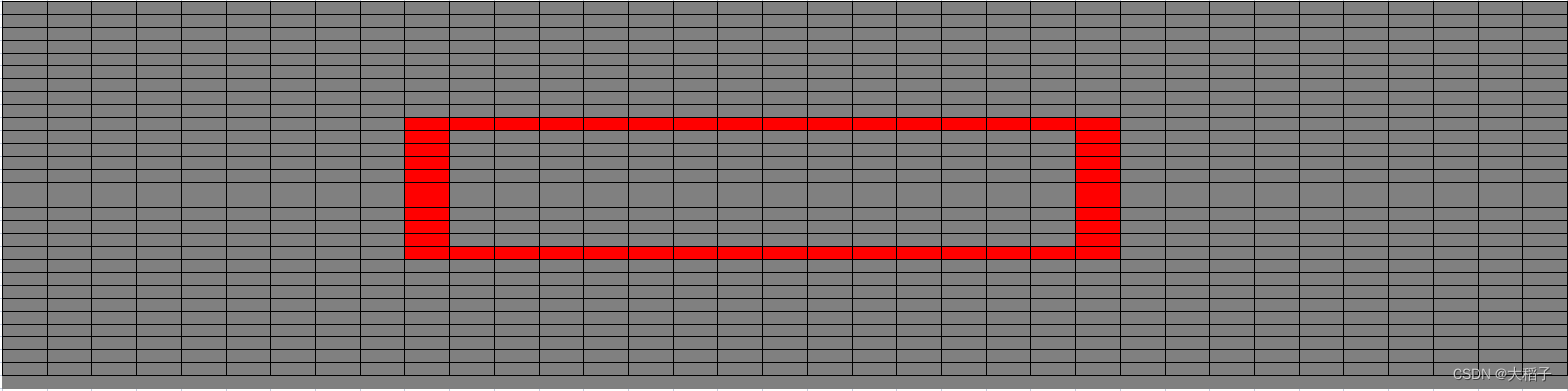
假定图像尺寸为(35，30，3), 图中存在文字标注框 text_box: [[10,10], [25,10], [25,20], [10,20]]，如下图所示，红色框即为文本标注框。
以此示例简单说明概率图、阈值图和二值化图的创建。
在这里插入图片描述

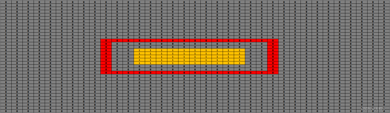
1.概率图标签

使用收缩的方式获取算法训练需要的概率图标签。
标注框内缩后，覆盖区域的概率值为1，其余区域概率值为0

# 创建概率图
h, w = 30, 35
probability_map = np.zeros((h, w), dtype=np.float32)
# 标注区域内缩 
# 经过distance的公式计算(D=2.52)和pyclipper库的内缩坐标处理
# text_box: [[10,10], [25,10], [25,20], [10,20]] ===> shrink_box: [[13,13], [22,13], [22,17], [13,17]]
# shrink_box为标注框经过内缩后的区域
shrink_box = [[13,13], [22,13], [22,17], [13,17]]
shrink_box = np.array(shrink_box).reshape(-1,2)
# 将概率图中的shrink区域赋值为1
cv2.fillPoly(probability_map, [shrink_box.astype(np.int32)], 1)

下图所示即为概率图，其中文字区域的概率值为1，背景区域的概率值为0
在这里插入图片描述

2.阈值图标签

阈值图中，需计算各位置到标注框的距离，距离越近的位置，阈值越高。
基本步骤如下：

(1) 标注框外扩

import pyclipper
import numpy as np
from shapely.geometry import Polygon

# 论文默认shrink值
r=0.4
# 标注框
subject = [[10,10],[25,10],[25,20],[10,20]]
# 创建Polygon对象
polygon = Polygon(subject)

# 计算偏置distance
distance = polygon.area*(1-np.power(r, 2))/polygon.length
print(distance)
# 2.52

# 创建PyclipperOffset对象
padding = pyclipper.PyclipperOffset()
# 向ClipperOffset对象添加一个路径用来准备偏置
padding.AddPath(subject, pyclipper.JT_MITER, pyclipper.ET_CLOSEDPOLYGON)

# polygon外扩
polygon_expand = padding.Execute(distance)[0]
polygon_expand = [tuple(l) for l in polygon_expand]
print(polygon_expand)
# [(7, 7), (28, 7), (28, 23), (7, 23)]

(2) 计算距离

标注框外扩后，文字区域扩大，需计算区域内每个点到标注框的距离。标注框看作四条线段，计算出每个位置点到这四条线段的距离，取最小值为最终距离。距离的计算借助两个三角形公式: 余弦定理和面积公式。具体的计算过程如下：

在这里插入图片描述
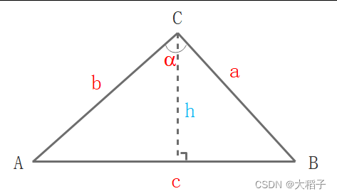
由三角形面积公式，推导出h：
$\begin{cases} S = \cfrac{1}{2}\cdot c \cdot h \\ S = \cfrac{1}{2}\cdot a \cdot b \cdot sin\alpha \end{cases} ⇒ h = \cfrac{a \cdot b}{c} \cdot sin\alpha$
其中，a, b和c的值可以通过位置距离计算， $sin\alpha$ 通过余弦定理计算得出：
$cos^2\alpha = \cfrac{a^2 + b^2 - c^2}{2ab} ⇒ sin\alpha = \sqrt{\smash[b]{1 - cos^2\alpha}}$

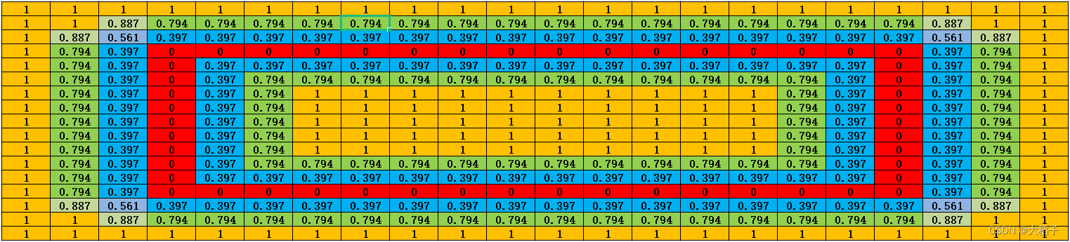
(3) 距离归一化

计算出每个位置点的值后，进行归一化。区域内所有的值除以前面计算出来的distance，限定取值在[0, 1]之间。得到相对距离比例的数值，如下图所示。
在这里插入图片描述

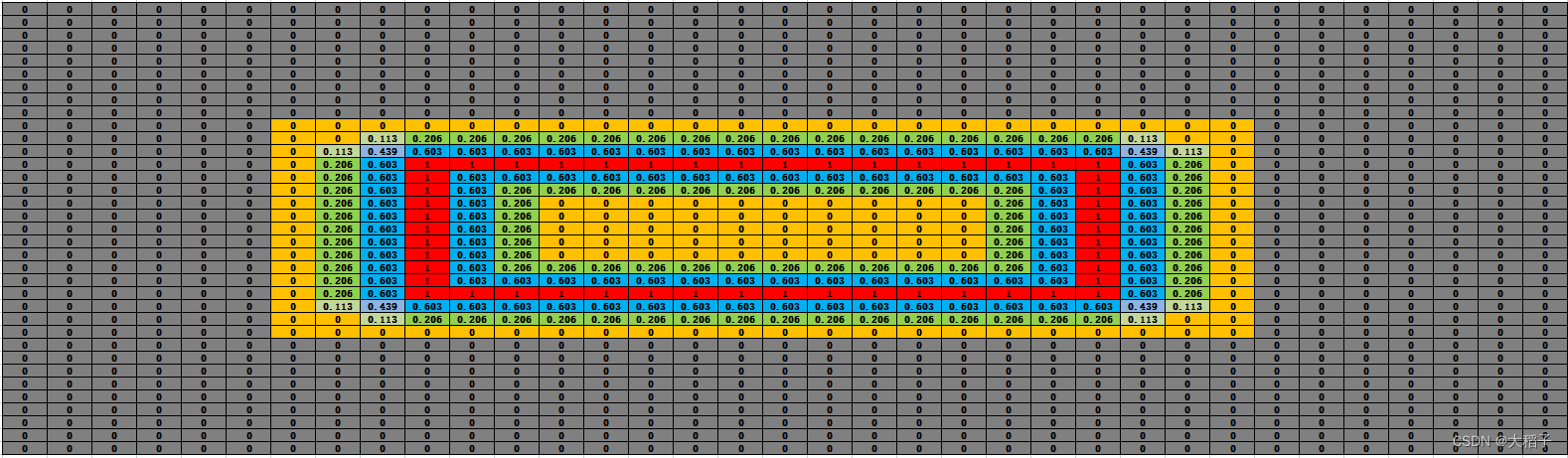
(4) 计算阈值图

用1减去距离归一化的值，即获取到阈值图。靠近标注框的位置，阈值接近1，阈值图如下所示。
在这里插入图片描述参照核心代码如下,详见paddleocr。

import cv2
import numpy as np
import pyclipper
from shapely.geometry import Polygon
from matplotlib import pyplot as plt 


class MakeBorderMap(object):
    def __init__(self,
                 shrink_ratio=0.4,
                 thresh_min=0.3,
                 thresh_max=0.7,
                 **kwargs):
        self.shrink_ratio = shrink_ratio
        self.thresh_min = thresh_min
        self.thresh_max = thresh_max

    def __call__(self, data):

        img = data['image']
        text_polys = data['polys']
        ignore_tags = data['ignore_tags']

        canvas = np.zeros(img.shape[:2], dtype=np.float32)
        mask = np.zeros(img.shape[:2], dtype=np.float32)

        for i in range(len(text_polys)):
            if ignore_tags[i]:
                continue
            self.draw_border_map(text_polys[i], canvas, mask=mask,data=data)
        #canvas = canvas * (self.thresh_max - self.thresh_min) + self.thresh_min

        data['threshold_map'] = canvas
        data['threshold_mask'] = mask
        return data

    def draw_border_map(self, polygon, canvas, mask, data):
        polygon = np.array(polygon)
        assert polygon.ndim == 2
        assert polygon.shape[1] == 2

        polygon_shape = Polygon(polygon)
        if polygon_shape.area <= 0:
            return
        distance = polygon_shape.area * (
            1 - np.power(self.shrink_ratio, 2)) / polygon_shape.length
        subject = [tuple(l) for l in polygon]
        padding = pyclipper.PyclipperOffset()
        #padding.AddPath(subject, pyclipper.JT_ROUND, pyclipper.ET_CLOSEDPOLYGON)
        padding.AddPath(subject, pyclipper.JT_MITER, pyclipper.ET_CLOSEDPOLYGON)

        padded_polygon = np.array(padding.Execute(distance)[0])
        cv2.fillPoly(mask, [padded_polygon.astype(np.int32)], 1.0)

        xmin = padded_polygon[:, 0].min()
        xmax = padded_polygon[:, 0].max()
        ymin = padded_polygon[:, 1].min()
        ymax = padded_polygon[:, 1].max()
        width = xmax - xmin + 1
        height = ymax - ymin + 1

        polygon[:, 0] = polygon[:, 0] - xmin
        polygon[:, 1] = polygon[:, 1] - ymin

        xs = np.broadcast_to(
            np.linspace(
                0, width - 1, num=width).reshape(1, width), (height, width))
        ys = np.broadcast_to(
            np.linspace(
                0, height - 1, num=height).reshape(height, 1), (height, width))

        distance_map = np.zeros(
            (polygon.shape[0], height, width), dtype=np.float32)
        for i in range(polygon.shape[0]):
            j = (i + 1) % polygon.shape[0]
            absolute_distance = self._distance(xs, ys, polygon[i], polygon[j])
            distance_map[i] = np.clip(absolute_distance / distance, 0, 1)
        distance_map = distance_map.min(axis=0)
        distance_map = np.round(distance_map, 3)
        data['distance_map'] = distance_map

        xmin_valid = min(max(0, xmin), canvas.shape[1] - 1)
        xmax_valid = min(max(0, xmax), canvas.shape[1] - 1)
        ymin_valid = min(max(0, ymin), canvas.shape[0] - 1)
        ymax_valid = min(max(0, ymax), canvas.shape[0] - 1)
        canvas[ymin_valid:ymax_valid + 1, xmin_valid:xmax_valid + 1] = np.fmax(
            1 - distance_map[ymin_valid - ymin:ymax_valid - ymax + height,
                             xmin_valid - xmin:xmax_valid - xmax + width],
            canvas[ymin_valid:ymax_valid + 1, xmin_valid:xmax_valid + 1])

    def _distance(self, xs, ys, point_1, point_2):
        '''
        compute the distance from point to a line
        ys: coordinates in the first axis
        xs: coordinates in the second axis
        point_1, point_2: (x, y), the end of the line
        '''
        height, width = xs.shape[:2]
        square_distance_1 = np.square(xs - point_1[0]) + np.square(ys - point_1[1])
        square_distance_2 = np.square(xs - point_2[0]) + np.square(ys - point_2[1])
        square_distance = np.square(point_1[0] - point_2[0]) + np.square(point_1[1] - point_2[1])

        cosin = (square_distance - square_distance_1 - square_distance_2) / (
            2 * np.sqrt(square_distance_1 * square_distance_2))
        square_sin = 1 - np.square(cosin)
        square_sin = np.nan_to_num(square_sin)
        result = np.sqrt(square_distance_1 * square_distance_2 * square_sin / square_distance)

        result[cosin < 0] = np.sqrt(np.fmin(square_distance_1, square_distance_2))[cosin< 0]
        return result

if __name__ == "__main__":
    data = dict()
    data['image'] = np.zeros((30, 35, 1), dtype=np.uint8)
    data['polys'] = [[[10,10],[25,10],[25,20],[10,20]]]
    data['ignore_tags'] = [False] 
    # 1. 声名MakeBorderMap函数
    generate_text_border = MakeBorderMap()
    
    # 2. 根据解码后的输入数据计算border
    data = generate_text_border(data)
    threshold_map = data['threshold_map']
    
    # 3. 阈值图可视化 
    plt.imshow(threshold_map)

在这里插入图片描述

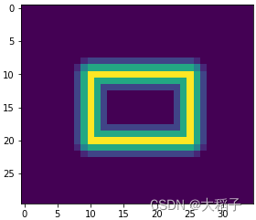
3.二值化图标签

三、损失计算

1. BCELoss损失函数

DBNet使用二分类交叉熵损失函数(binary cross-entropy)，并且是单标签的，即一个输入样本对应于一个分类输出（1或0）。对于包含N个样本的数据D(x, y)，BCE损失计算公式如下：
$=\frac{1}{N} \sum_{\mathclap{1\le i\le n}} l_i$
其中， $l_i = -w(y_i\cdot \log x_i + (1-y_i)*\log(1-x_i))$ 为第i个样本对应的loss。 $w$ 是超参数，对于单标签二分类，设不设置 $w$ 没有影响。第i个样本的损失为：
$l_i = \begin{cases} -\log x_i &\text{if } & y=1 \\ -\log(1-x_i) &\text{if } & y=0 \end{cases}$

2. 二值化函数

(1) 标准二值化

语义分割网络生成概率图 $P\in R^{H*W}$ ，其中 $H$ 和 $W$ 分别代表高度和宽度。概率图需要转换成二值化图，像素值为1的地方代表文字区域。标准二值化过程如下：
$B_{i,j} = \begin{cases} 1 &\text{if } &P_{i,j}>=t \\ 0 &\text{if } &otherwise \end{cases}$
其中， $t$ 是固定的阈值， $(i, j)$ 代表图上的坐标。

(2) 可微分二值化

标准二值化函数是不连续的，其过程是不可微的，不能随着语义分割网络的训练而优化。为了解决这个问题，论文提出了一个近似二值化过程的阶跃函数，即可微分二值化(Differentiable binarization)，其过程如下：
$\^{B}_{i,j} = \frac{1}{1+e^{-k(P_{i,j}-T_{i,j})}}$
其中， $\^{B}$ 是输出的二值化图， $T$ 是网络学到的自适应阈值图， $k$ 表示放大因子，通常设置为50。
下图(a)中SB表示标准二值化过程，DB表示可微分二值化过程；图(b)和图©分别表示 $l_+$ 和 $l_-$ 的导数曲线

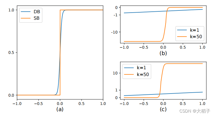
DBNet提升效果的原因可以通过反向梯度传播解释。在BCELoss中，定义 $f(x)=\frac{1}{1+e^{-kx}}$ ，其中 $x=P_{i,j}-T_{i,j}$ 。则正样本损失和负样本损失计算如下:
$\begin{cases} l_+ = - \log \frac{1}{1+e^{-kx}} \\ l_- = - \log (1- \frac{1}{1+e^{-kx}}) \end{cases}$
loss对于x的偏导数计算如下：
$\begin{cases} \frac{\partial l_+}{\partial x} = -kf(x)e^{-kx} \\ \frac{\partial l_-}{\partial x} = kf(x) \end{cases}$
通过偏导数我们可以注意到：

(1) 错误预测的梯度通过增强因子 $k$ 被加强，更利于网络的优化学习，使预测结果更清晰
(2) 图(b)为 $l_+$ 的导数曲线，如果发生误报(正样本被预测为负样本，即x<0), 图(b)中小于0的部分导数值非常大，说明损失也非常大，则更能清晰的进行梯度回传
(3) 图©为 $l_-$ 的导数曲线，如果发生误报(负样本被预测为正样本，即x>0), 梯度也比较大，损失也很大

3. 整体损失计算

模型训练过程中输出三个图：概率图、阈值图和二值化图。从而在损失函数计算时，也要结合这3个图与它们对应的真实标签构建3部分损失函数。总的损失函数公式定义如下：
$L=L_s + ɑ×L_b + β×L_t$
其中，L为总的损失， $L_s$ 为概率图损失， $L_b$ 为二值化图损失， $L_t$ 为阈值图损失。 $ɑ$ 和 $β$ 为权重系数，论文中分别设置为1和10。
$L_s = L_b = \sum_{\mathclap{i \in S_l}} y_i \log x_i + (1-y_i)\log(1-x_i)$
对于 $L_s$ 和 $L_b$ 的损失计算都使用BCELoss, 为了解决正负样本不均衡的问题，在损失计算过程中使用错题集策略，同时正负样本比例设为1：3。
$L_t$ 计算方式为扩展多边形 $G_d$ 内预测结果和阈值图标签的L1距离之和。
$L_t = \sum_{\mathclap{i \in R_d}} |{y_i}^* - {x_i}^*|$
其中， $R_d$ 是扩展多边形 $G_d$ 内的像素索引， $y^*$ 是阈值图标签。

【DBNet模型】