基于MATLAB的CT滤波反投影算法的实验研究

实验四 滤波反投影算法的实验研究
1、利用”iradon”函数采用S-L与R-L滤波器进行滤波实现滤波反投影算法。

I=phantom(256);
theta=0:1:179;
P=radon(I,theta);
rec=iradon(P,theta,'linear','None');
rec_RL=iradon(P,theta,'Ram-Lak');
rec_SL=iradon(P,theta,'linear','Shepp-Logan');
figure;
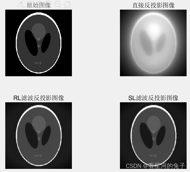
subplot(2,2,1);imshow(I,[]),title('原始图像');
subplot(2,2,2);imshow(rec,[]),title('直接反投影图像');
subplot(2,2,3);imshow(rec_RL,[]),title('RL滤波反投影图像');
subplot(2,2,4);imshow(rec_SL,[]),title('SL滤波反投影图像');

2、利用FBP算法重建图像
1）对椭圆平行束投影数据进行滤波反投影重建，分别采用S-L与R-L滤波器进行滤波

clear;
N=256;
I = phantom('Shepp-Logan',N);
delta=pi/180;
theta=0:1:179;
theta_num=length(theta);
d=1;
%%产生投影数据
P=radon(I,theta);
[mm,nn]=size(P);
e=floor((mm-N-1)/2+1)+1;
P=P(e:N+e-1,:);
P1=reshape(P,N,theta_num);
%%
fh_RL=medfuncRlfilterfunction(N,d);
fh_SL=medfuncSlfilterfunction(N,d);
%%
rec=zeros(N);
for m=1:theta_num
    pm=P1(:,m);
    Cm=(N/2)*(1-cos((m-1)*delta)-sin((m-1)*delta));
    for k1=1:N
        for k2=1:N
            Xrm=Cm+(k2-1)*cos((m-1)*delta)+(k1-1)*sin((m-1)*delta);
            n=floor(Xrm);
            t=Xrm-floor(Xrm);
            n=max(1,n);
            n=min(n,N-1);
            p=(1-t)*pm(n)+t*pm(n+1);
            rec(N+1-k1,k2)=rec(N+1-k1,k2)+p;
        end
    end
end
%%
rec_RL=zeros(N)
for m1=1:theta_num
    pm1=P1(:,m1);
    pm_RL=conv(fh_RL,pm1,'same');
    Cm1=(N/2)*(1-cos((m1-1)*delta)-sin((m1-1)*delta));
    for k1=1:N
        for k2=1:N
            Xrm1=Cm1+(k2-1)*cos((m1-1)*delta)+(k1-1)*sin((m1-1)*delta);
            n1=floor(Xrm1);
            t1=Xrm1-floor(Xrm1);
            n1=max(1,n1);
            n1=min(n1,N-1);
            p1=(1-t1)*pm_RL(n1)+t1*pm_RL(n1+1);
            rec_RL(N+1-k1,k2)=rec_RL(N+1-k1,k2)+p1;
        end
    end
end
%%
rec_SL=zeros(N)
for m2=1:theta_num
    pm2=P1(:,m2);
    pm_SL=conv(fh_SL,pm2,'same');
    Cm2=(N/2)*(1-cos((m2-1)*delta)-sin((m2-1)*delta));
    for k1=1:N
        for k2=1:N
            Xrm2=Cm2+(k2-1)*cos((m2-1)*delta)+(k1-1)*sin((m2-1)*delta);
            n2=floor(Xrm2);
            t2=Xrm2-floor(Xrm2);
            n2=max(1,n2);
            n2=min(n2,N-1);
            p2=(1-t2)*pm_SL(n2)+t2*pm_SL(n2+1);
            rec_SL(N+1-k1,k2)=rec_SL(N+1-k1,k2)+p2;
        end
    end
end
%%
figure;
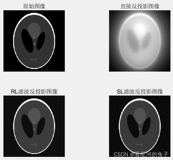
subplot(2,2,1);imshow(I,[]),title('原始图像');
subplot(2,2,2);imshow(rec,[]),title('直接反投影图像');
subplot(2,2,3);imshow(rec_RL,[]),title('RL滤波反投影图像');
subplot(2,2,4);imshow(rec_SL,[]),title('SL滤波反投影图像');

2）对Shepp-Logan图平行束投影数据进行滤波反投影重建，别采用S-L与R-L滤波器进行滤波

clear;
N=256;
I=phantom(N);
delta=pi/180;
theta=0:1:179;
theta_num=length(theta);
d=1;
%%产生投影数据
P=radon(I,theta);
[mm,nn]=size(P);
e=floor((mm-N-1)/2+1)+1;
P=P(e:N+e-1,:);
P1=reshape(P,N,theta_num);
%%
fh_RL=medfuncRlfilterfunction(N,d);
fh_SL=medfuncSlfilterfunction(N,d);
%%
rec=zeros(N);
for m=1:theta_num
    pm=P1(:,m);
    Cm=(N/2)*(1-cos((m-1)*delta)-sin((m-1)*delta));
    for k1=1:N
        for k2=1:N
            Xrm=Cm+(k2-1)*cos((m-1)*delta)+(k1-1)*sin((m-1)*delta);
            n=floor(Xrm);
            t=Xrm-floor(Xrm);
            n=max(1,n);
            n=min(n,N-1);
            p=(1-t)*pm(n)+t*pm(n+1);
            rec(N+1-k1,k2)=rec(N+1-k1,k2)+p;
        end
    end
end
%%
rec_RL=zeros(N)
for m1=1:theta_num
    pm1=P1(:,m1);
    pm_RL=conv(fh_RL,pm1,'same');
    Cm1=(N/2)*(1-cos((m1-1)*delta)-sin((m1-1)*delta));
    for k1=1:N
        for k2=1:N
            Xrm1=Cm1+(k2-1)*cos((m1-1)*delta)+(k1-1)*sin((m1-1)*delta);
            n1=floor(Xrm1);
            t1=Xrm1-floor(Xrm1);
            n1=max(1,n1);
            n1=min(n1,N-1);
            p1=(1-t1)*pm_RL(n1)+t1*pm_RL(n1+1);
            rec_RL(N+1-k1,k2)=rec_RL(N+1-k1,k2)+p1;
        end
    end
end
%%
rec_SL=zeros(N)
for m2=1:theta_num
    pm2=P1(:,m2);
    pm_SL=conv(fh_SL,pm2,'same');
    Cm2=(N/2)*(1-cos((m2-1)*delta)-sin((m2-1)*delta));
    for k1=1:N
        for k2=1:N
            Xrm2=Cm2+(k2-1)*cos((m2-1)*delta)+(k1-1)*sin((m2-1)*delta);
            n2=floor(Xrm2);
            t2=Xrm2-floor(Xrm2);
            n2=max(1,n2);
            n2=min(n2,N-1);
            p2=(1-t2)*pm_SL(n2)+t2*pm_SL(n2+1);
            rec_SL(N+1-k1,k2)=rec_SL(N+1-k1,k2)+p2;
        end
    end
end
%%
figure;
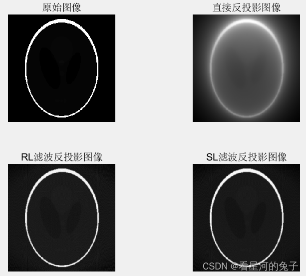
subplot(2,2,1);imshow(I,[]),title('原始图像');
subplot(2,2,2);imshow(rec,[]),title('直接反投影图像');
subplot(2,2,3);imshow(rec_RL,[]),title('RL滤波反投影图像');
subplot(2,2,4);imshow(rec_SL,[]),title('SL滤波反投影图像');