3-1 jupyter notebook基础
Notbook 示例

Notbook 源码
[1]
for x in range(5):
    print('hello world')
hello world
hello world
hello world
hello world
hello world

欢迎来到机器学习
阿济格的回复考核

[2]
 data = [ 2*i for i in range(100) ]
print(data)
[0, 2, 4, 6, 8, 10, 12, 14, 16, 18, 20, 22, 24, 26, 28, 30, 32, 34, 36, 38, 40, 42, 44, 46, 48, 50, 52, 54, 56, 58, 60, 62, 64, 66, 68, 70, 72, 74, 76, 78, 80, 82, 84, 86, 88, 90, 92, 94, 96, 98, 100, 102, 104, 106, 108, 110, 112, 114, 116, 118, 120, 122, 124, 126, 128, 130, 132, 134, 136, 138, 140, 142, 144, 146, 148, 150, 152, 154, 156, 158, 160, 162, 164, 166, 168, 170, 172, 174, 176, 178, 180, 182, 184, 186, 188, 190, 192, 194, 196, 198]

[3]
data[-1]
198
变量一旦在jupyer notebook 中创建即被保存

[4]
len(data)
100
[8]
data[:10]
[0, 2, 4, 6, 8, 10, 12, 14, 16, 18]
[6]
print(5464654)
5464654
3-2 jupyter notebook中的魔法命令
Notbook 示例
Notbook 源码
[1]
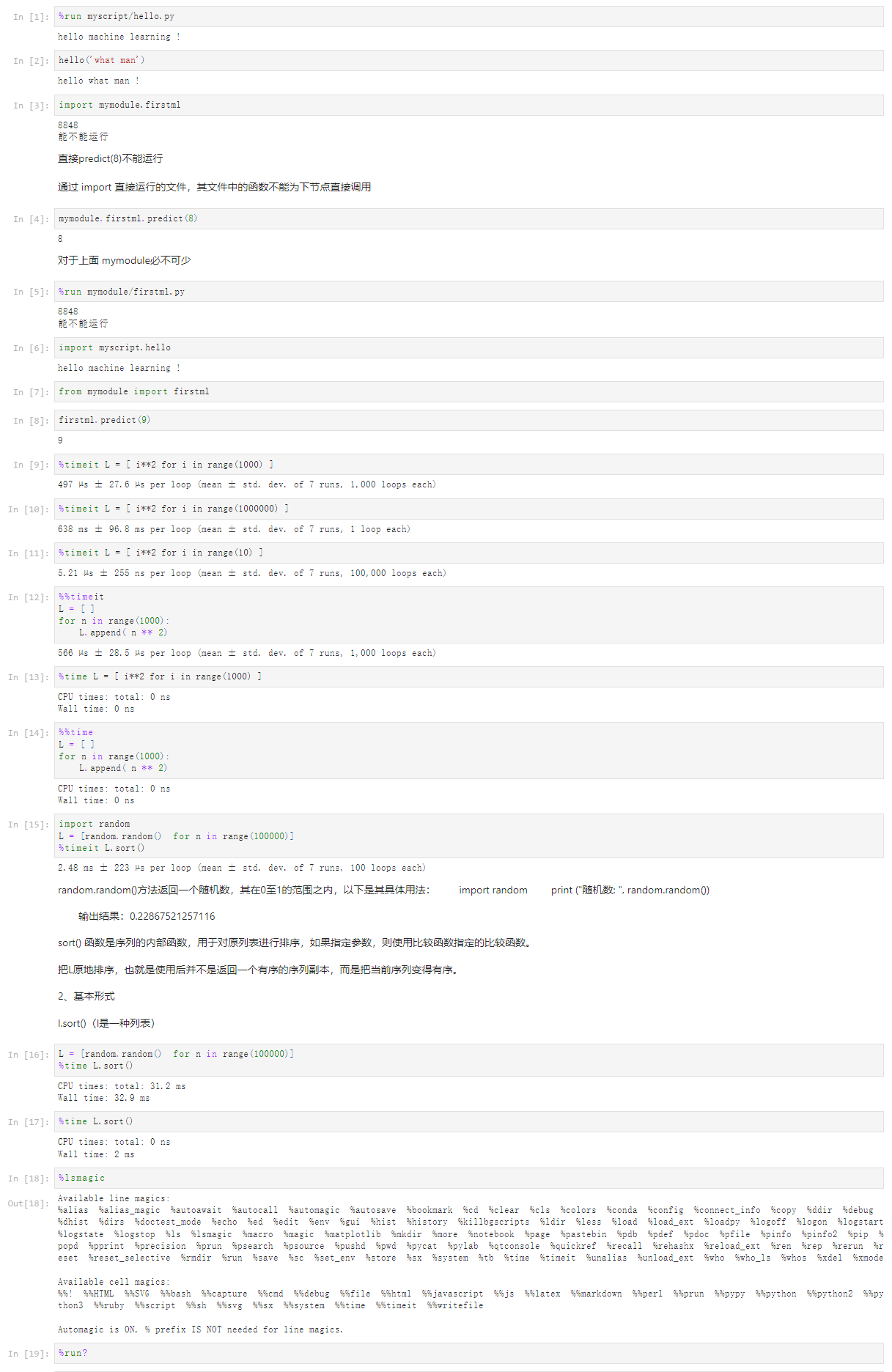
%run myscript/hello.py
hello machine learning !
[2]
hello('what man')
hello what man !
[3]
import mymodule.firstml
8848
能不能运行
直接predict(8)不能运行
通过 import 直接运行的文件,其文件中的函数不能为下节点直接调用
[4]
mymodule.firstml.predict(8)
8
对于上面 mymodule必不可少
[5]
%run mymodule/firstml.py
8848
能不能运行
[6]
import myscript.hello
hello machine learning !
[7]
from mymodule import firstml
[8]
firstml.predict(9)
9
[9]
%timeit L = [ i**2 for i in range(1000) ]
497 µs ± 27.6 µs per loop (mean ± std. dev. of 7 runs, 1,000 loops each)
[10]
%timeit L = [ i**2 for i in range(1000000) ]
638 ms ± 96.8 ms per loop (mean ± std. dev. of 7 runs, 1 loop each)
[11]
%timeit L = [ i**2 for i in range(10) ]
5.21 µs ± 255 ns per loop (mean ± std. dev. of 7 runs, 100,000 loops each)
[12]
%%timeit
L = [ ]
for n in range(1000):
L.append( n ** 2)
566 µs ± 28.5 µs per loop (mean ± std. dev. of 7 runs, 1,000 loops each)
[13]
%time L = [ i**2 for i in range(1000) ]
CPU times: total: 0 ns
Wall time: 0 ns
[14]
%%time
L = [ ]
for n in range(1000):
L.append( n ** 2)
CPU times: total: 0 ns
Wall time: 0 ns
[15]
import random
L = [random.random() for n in range(100000)]
%timeit L.sort()
2.48 ms ± 223 µs per loop (mean ± std. dev. of 7 runs, 100 loops each)
random.random()方法返回一个随机数,其在0至1的范围之内,以下是其具体用法: import random print ("随机数: ", random.random())
输出结果:0.22867521257116
sort() 函数是序列的内部函数,用于对原列表进行排序,如果指定参数,则使用比较函数指定的比较函数。
把L原地排序,也就是使用后并不是返回一个有序的序列副本,而是把当前序列变得有序。
2、基本形式
l.sort()(l是一种列表)
[16]
L = [random.random() for n in range(100000)]
%time L.sort()
CPU times: total: 31.2 ms
Wall time: 32.9 ms
[17]
%time L.sort()
CPU times: total: 0 ns
Wall time: 2 ms
[18]
%lsmagic
Available line magics:
%alias %alias_magic %autoawait %autocall %automagic %autosave %bookmark %cd %clear %cls %colors %conda %config %connect_info %copy %ddir %debug %dhist %dirs %doctest_mode %echo %ed %edit %env %gui %hist %history %killbgscripts %ldir %less %load %load_ext %loadpy %logoff %logon %logstart %logstate %logstop %ls %lsmagic %macro %magic %matplotlib %mkdir %more %notebook %page %pastebin %pdb %pdef %pdoc %pfile %pinfo %pinfo2 %pip %popd %pprint %precision %prun %psearch %psource %pushd %pwd %pycat %pylab %qtconsole %quickref %recall %rehashx %reload_ext %ren %rep %rerun %reset %reset_selective %rmdir %run %save %sc %set_env %store %sx %system %tb %time %timeit %unalias %unload_ext %who %who_ls %whos %xdel %xmode
Available cell magics:
%%! %%HTML %%SVG %%bash %%capture %%cmd %%debug %%file %%html %%javascript %%js %%latex %%markdown %%perl %%prun %%pypy %%python %%python2 %%python3 %%ruby %%script %%sh %%svg %%sx %%system %%time %%timeit %%writefile
Automagic is ON, % prefix IS NOT needed for line magics.
[19]
%run?
3-3 Numpy数据基础and3-4 创建numpy数组和矩阵
Notbook 示例
Notbook 源码
[1]
import numpy
[2]
numpy.__version__
'1.21.5'
[3]
import numpy as np
[4]
np.__version__
'1.21.5'
python list 的特点

[5]
L = [ i for i in range(10)]
L
[0, 1, 2, 3, 4, 5, 6, 7, 8, 9]
[6]
L[5]
5
[7]
L[5] = 100
L
[0, 1, 2, 3, 4, 100, 6, 7, 8, 9]
[8]
L[5] = 'machine learning'
L
[0, 1, 2, 3, 4, 'machine learning', 6, 7, 8, 9]
上面单双引号均可

[9]
import array
[10]
arr = array.array('i',[ i for i in range(10)])
arr
array('i', [0, 1, 2, 3, 4, 5, 6, 7, 8, 9])
[11]
arr[5]
5
[12]
arr[5] = 100
arr[5]
100
arr[5] = 'machine learing '报错 array.array,限定数据类型。限制了灵活性,相对速度比较高;同时array只是将存储的数据看成数组或二维数组,而数组并没有看成矩阵,也没有配备向量或矩阵相关的运算; myArray = array.array('i', [i for i range(10)])

numpy.array
[13]
nparr = np.array([i for i in range(10)])
nparr
array([0, 1, 2, 3, 4, 5, 6, 7, 8, 9])
[14]
nparr[5]
5
[15]
nparr[5] = 10
nparr
array([ 0,  1,  2,  3,  4, 10,  6,  7,  8,  9])
nparry[5] = "machine learning" 将报错

[16]
nparr.dtype
dtype('int32')
[17]
nparr[5] = 5.0
[18]
nparr
array([0, 1, 2, 3, 4, 5, 6, 7, 8, 9])
[19]
nparr.dtype
dtype('int32')
[20]
nparr[5] = 3.14
nparr
array([0, 1, 2, 3, 4, 3, 6, 7, 8, 9])
[21]
nparr2 = np.array([1, 2, 3.0])
nparr2.dtype
dtype('float64')
[22]
np.zeros(10)
array([0., 0., 0., 0., 0., 0., 0., 0., 0., 0.])
[23]
np.zeros(10).dtype
dtype('float64')
[24]
np.zeros(10,dtype = int)
array([0, 0, 0, 0, 0, 0, 0, 0, 0, 0])
[25]
np.zeros((3,5))
array([[0., 0., 0., 0., 0.],
       [0., 0., 0., 0., 0.],
       [0., 0., 0., 0., 0.]])
[58]
np.zeros(shape = (3,5),dtype = int)
array([[0, 0, 0, 0, 0],
       [0, 0, 0, 0, 0],
       [0, 0, 0, 0, 0]])
[27]
np.ones(10)
array([1., 1., 1., 1., 1., 1., 1., 1., 1., 1.])
[28]
np.ones((3,5))
array([[1., 1., 1., 1., 1.],
       [1., 1., 1., 1., 1.],
       [1., 1., 1., 1., 1.]])
[29]
np.full((3,6),666)
array([[666, 666, 666, 666, 666, 666],
       [666, 666, 666, 666, 666, 666],
       [666, 666, 666, 666, 666, 666]])
[30]
np.full(shape = (3,6),fill_value = 666)
array([[666, 666, 666, 666, 666, 666],
       [666, 666, 666, 666, 666, 666],
       [666, 666, 666, 666, 666, 666]])
fill_value 只有一个下划线

[31]
np.full(fill_value = 666,shape = (3,6))
array([[666, 666, 666, 666, 666, 666],
       [666, 666, 666, 666, 666, 666],
       [666, 666, 666, 666, 666, 666]])
[32]
np.full(fill_value = 6,shape = (10))
array([6, 6, 6, 6, 6, 6, 6, 6, 6, 6])
[33]
[i for i in range(0,20,2)]
[0, 2, 4, 6, 8, 10, 12, 14, 16, 18]
[34]
np.arange(0,20,2)
array([ 0,  2,  4,  6,  8, 10, 12, 14, 16, 18])
[35]
np.arange(0,1,0.2)
array([0. , 0.2, 0.4, 0.6, 0.8])
在python中range步长只能为整数

[36]
np.arange(0,10)
array([0, 1, 2, 3, 4, 5, 6, 7, 8, 9])
[37]
np.arange(10)
array([0, 1, 2, 3, 4, 5, 6, 7, 8, 9])
linspace
[38]
np.linspace(0,20,10)
array([ 0.        ,  2.22222222,  4.44444444,  6.66666667,  8.88888889,
       11.11111111, 13.33333333, 15.55555556, 17.77777778, 20.        ])
[39]
np.linspace(0,20,11)
array([ 0.,  2.,  4.,  6.,  8., 10., 12., 14., 16., 18., 20.])
random
[40]
np.random.randint(0,10)
6
[41]
np.random.randint(0,10,10)
array([7, 0, 8, 7, 7, 4, 1, 4, 4, 8])
前闭后开,对于上面永远娶不到10

[42]
np.random.randint(0,1,10)
array([0, 0, 0, 0, 0, 0, 0, 0, 0, 0])
[43]
np.random.randint(4,8,size = 10)
array([7, 6, 6, 7, 5, 6, 4, 6, 5, 7])
[44]
np.random.randint(4,8,size = (3,5))
array([[4, 4, 5, 7, 6],
       [7, 7, 4, 7, 7],
       [6, 5, 5, 6, 7]])
[45]
np.random.randint(4,8,size = (3,5))
array([[7, 4, 6, 6, 6],
       [7, 4, 5, 6, 5],
       [4, 4, 6, 6, 7]])
[46]
np.random.seed(666)
[47]
np.random.randint(4,8,size = (3,5))
array([[4, 6, 5, 6, 6],
       [6, 5, 6, 4, 5],
       [7, 6, 7, 4, 7]])
[48]
np.random.seed(666)
np.random.randint(4,8,size = (3,5))
array([[4, 6, 5, 6, 6],
       [6, 5, 6, 4, 5],
       [7, 6, 7, 4, 7]])
[49]
np.random.random()
0.2811684913927954
最后一个random必须加括号

[50]
np.random.random(10)
array([0.46284169, 0.23340091, 0.76706421, 0.81995656, 0.39747625,
       0.31644109, 0.15551206, 0.73460987, 0.73159555, 0.8578588 ])
[51]
np.random.random((3,5))
array([[0.76741234, 0.95323137, 0.29097383, 0.84778197, 0.3497619 ],
       [0.92389692, 0.29489453, 0.52438061, 0.94253896, 0.07473949],
       [0.27646251, 0.4675855 , 0.31581532, 0.39016259, 0.26832981]])
[52]
np.random.normal()
0.7760516793129695
[53]
np.random.normal(10,100)
128.06359754812632
均值为10,方差为100

[54]
np.random.normal(0,1,(3,5))
array([[ 0.06102404,  1.07856138, -0.79783572,  1.1701326 ,  0.1121217 ],
       [ 0.03185388, -0.19206285,  0.78611284, -1.69046314, -0.98873907],
       [ 0.31398563,  0.39638567,  0.57656584, -0.07019407,  0.91250436]])
[59]
np.random.normal?
[60]
np.random?
[57]
help(np.random.normal)
Help on built-in function normal:

normal(...) method of numpy.random.mtrand.RandomState instance
    normal(loc=0.0, scale=1.0, size=None)

    Draw random samples from a normal (Gaussian) distribution.

    The probability density function of the normal distribution, first
    derived by De Moivre and 200 years later by both Gauss and Laplace
    independently [2]_, is often called the bell curve because of
    its characteristic shape (see the example below).

    The normal distributions occurs often in nature.  For example, it
    describes the commonly occurring distribution of samples influenced
    by a large number of tiny, random disturbances, each with its own
    unique distribution [2]_.

    .. note::
        New code should use the ``normal`` method of a ``default_rng()``
        instance instead; please see the :ref:`random-quick-start`.

    Parameters
    ----------
    loc : float or array_like of floats
        Mean ("centre") of the distribution.
    scale : float or array_like of floats
        Standard deviation (spread or "width") of the distribution. Must be
        non-negative.
    size : int or tuple of ints, optional
        Output shape.  If the given shape is, e.g., ``(m, n, k)``, then
        ``m * n * k`` samples are drawn.  If size is ``None`` (default),
        a single value is returned if ``loc`` and ``scale`` are both scalars.
        Otherwise, ``np.broadcast(loc, scale).size`` samples are drawn.

    Returns
    -------
    out : ndarray or scalar
        Drawn samples from the parameterized normal distribution.

    See Also
    --------
    scipy.stats.norm : probability density function, distribution or
        cumulative density function, etc.
    Generator.normal: which should be used for new code.

    Notes
    -----
    The probability density for the Gaussian distribution is

    .. math:: p(x) = \frac{1}{\sqrt{ 2 \pi \sigma^2 }}
                     e^{ - \frac{ (x - \mu)^2 } {2 \sigma^2} },

    where :math:`\mu` is the mean and :math:`\sigma` the standard
    deviation. The square of the standard deviation, :math:`\sigma^2`,
    is called the variance.

    The function has its peak at the mean, and its "spread" increases with
    the standard deviation (the function reaches 0.607 times its maximum at
    :math:`x + \sigma` and :math:`x - \sigma` [2]_).  This implies that
    normal is more likely to return samples lying close to the mean, rather
    than those far away.

    References
    ----------
    .. [1] Wikipedia, "Normal distribution",
           https://en.wikipedia.org/wiki/Normal_distribution
    .. [2] P. R. Peebles Jr., "Central Limit Theorem" in "Probability,
           Random Variables and Random Signal Principles", 4th ed., 2001,
           pp. 51, 51, 125.

    Examples
    --------
    Draw samples from the distribution:

    >>> mu, sigma = 0, 0.1 # mean and standard deviation
    >>> s = np.random.normal(mu, sigma, 1000)

    Verify the mean and the variance:

    >>> abs(mu - np.mean(s))
    0.0  # may vary

    >>> abs(sigma - np.std(s, ddof=1))
    0.1  # may vary

    Display the histogram of the samples, along with
    the probability density function:

    >>> import matplotlib.pyplot as plt
    >>> count, bins, ignored = plt.hist(s, 30, density=True)
    >>> plt.plot(bins, 1/(sigma * np.sqrt(2 * np.pi)) *
    ...                np.exp( - (bins - mu)**2 / (2 * sigma**2) ),
    ...          linewidth=2, color='r')
    >>> plt.show()

    Two-by-four array of samples from N(3, 6.25):

    >>> np.random.normal(3, 2.5, size=(2, 4))
    array([[-4.49401501,  4.00950034, -1.81814867,  7.29718677],   # random
           [ 0.39924804,  4.68456316,  4.99394529,  4.84057254]])  # random
3-5 Numpy数组的基本操作and3-6 Numpy数组的合并与分割
Notbook 示例
Notbook 源码
[1]
import numpy as np
[2]
x = np.arange(10)
x
array([0, 1, 2, 3, 4, 5, 6, 7, 8, 9])
[3]
X = np.arange(15).reshape(3,5)
X
array([[ 0, 1, 2, 3, 4],
[ 5, 6, 7, 8, 9],
[10, 11, 12, 13, 14]])
基本属性
[4]
x.ndim
1
[5]
X.ndim
2
[6]
x.shape
(10,)
[7]
X.shape
(3, 5)
[8]
x.size
10
[9]
X.size
15
Numpy.array的数据访问
[10]
x
array([0, 1, 2, 3, 4, 5, 6, 7, 8, 9])
[11]
x[0]
0
[12]
x[-1]
9
[13]
X
array([[ 0, 1, 2, 3, 4],
[ 5, 6, 7, 8, 9],
[10, 11, 12, 13, 14]])
[14]
X[0][0]
0
[15]
X[(2,2)]
12
[16]
X[2,2]
12
[17]
X[2][2]
12
[18]
X[:2][:2]
array([[0, 1, 2, 3, 4],
[5, 6, 7, 8, 9]])
注意与切片方式区分
[19]
x[0:5]
array([0, 1, 2, 3, 4])
[20]
x[:5]
array([0, 1, 2, 3, 4])
[21]
x[5:]
array([5, 6, 7, 8, 9])
[22]
x[::2]
array([0, 2, 4, 6, 8])
[23]
x[::-1]
array([9, 8, 7, 6, 5, 4, 3, 2, 1, 0])
[24]
X
array([[ 0, 1, 2, 3, 4],
[ 5, 6, 7, 8, 9],
[10, 11, 12, 13, 14]])
[25]
X[:2,:3]
array([[0, 1, 2],
[5, 6, 7]])
[26]
x
array([0, 1, 2, 3, 4, 5, 6, 7, 8, 9])
[27]
x[:2][:3]
array([0, 1])
[28]
X[:2][:3]
array([[0, 1, 2, 3, 4],
[5, 6, 7, 8, 9]])
[29]
X[:2]
array([[0, 1, 2, 3, 4],
[5, 6, 7, 8, 9]])
[30]
X[:2][:3]
array([[0, 1, 2, 3, 4],
[5, 6, 7, 8, 9]])
X[:2][:3]在X[:2]的基础上取值,还是按行取,欲取三个只有两个,故全部取出
[31]
X
array([[ 0, 1, 2, 3, 4],
[ 5, 6, 7, 8, 9],
[10, 11, 12, 13, 14]])
[32]
X[:2,::2] #::2
array([[0, 2, 4],
[5, 7, 9]])
[33]
X[::-1,::-1]
array([[14, 13, 12, 11, 10],
[ 9, 8, 7, 6, 5],
[ 4, 3, 2, 1, 0]])
[34]
X[0]
array([0, 1, 2, 3, 4])
[35]
X[0,::] #对于此行及以下三行,:与::效果相同
array([0, 1, 2, 3, 4])
[36]
X[::,0]
array([ 0, 5, 10])
[37]
X[0,::].ndim
1
[38]
X[::,0]
array([ 0, 5, 10])
[39]
X[:,0].ndim
1
[40]
subx = X[:2,:3]
subx
array([[0, 1, 2],
[5, 6, 7]])
[41]
subx[0][0]=100
subx
array([[100, 1, 2],
[ 5, 6, 7]])
[42]
X
array([[100, 1, 2, 3, 4],
[ 5, 6, 7, 8, 9],
[ 10, 11, 12, 13, 14]])
相对于python 创建一个子矩阵,numpy则直接引用
[43]
X[0][0] = 0
X
array([[ 0, 1, 2, 3, 4],
[ 5, 6, 7, 8, 9],
[10, 11, 12, 13, 14]])
[44]
subx
array([[0, 1, 2],
[5, 6, 7]])
[45]
subx = X[:2,:3].copy()
subx
array([[0, 1, 2],
[5, 6, 7]])
[46]
subx[0][0] = 100
subx
array([[100, 1, 2],
[ 5, 6, 7]])
[47]
X
array([[ 0, 1, 2, 3, 4],
[ 5, 6, 7, 8, 9],
[10, 11, 12, 13, 14]])
reshape
[48]
x.shape
(10,)
[49]
x.ndim
1
[50]
x.reshape(2,5)
array([[0, 1, 2, 3, 4],
[5, 6, 7, 8, 9]])
[51]
x
array([0, 1, 2, 3, 4, 5, 6, 7, 8, 9])
[52]
A = x.reshape(2,5)
A
array([[0, 1, 2, 3, 4],
[5, 6, 7, 8, 9]])
[53]
x
array([0, 1, 2, 3, 4, 5, 6, 7, 8, 9])
[54]
B = x.reshape(1,10)
B
array([[0, 1, 2, 3, 4, 5, 6, 7, 8, 9]])
[55]
B.ndim
2
[56]
B.shape
(1, 10)
[57]
x.shape
(10,)
[58]
x.reshape(10,-1)
array([[0],
[1],
[2],
[3],
[4],
[5],
[6],
[7],
[8],
[9]])
[59]
x.reshape(-1,10)
array([[0, 1, 2, 3, 4, 5, 6, 7, 8, 9]])
[60]
x.reshape(2,-1)
array([[0, 1, 2, 3, 4],
[5, 6, 7, 8, 9]])
合并操作
[61]
x = np.array([1,2,3])
y = np.array([3,2,1])
[62]
x
array([1, 2, 3])
[63]
y
array([3, 2, 1])
[64]
np.concatenate([x,y])
array([1, 2, 3, 3, 2, 1])
[65]
z = np.array([666,666,666])
[66]
np.concatenate([x,y,z])
array([ 1, 2, 3, 3, 2, 1, 666, 666, 666])
[67]
A = np.array([[1,2,3],[4,5,6]])
A
array([[1, 2, 3],
[4, 5, 6]])
[68]
np.concatenate([A,A])
array([[1, 2, 3],
[4, 5, 6],
[1, 2, 3],
[4, 5, 6]])
[69]
np.concatenate([A,A],axis = 1)
array([[1, 2, 3, 1, 2, 3],
[4, 5, 6, 4, 5, 6]])
[70]
np.concatenate([A,A],axis = 0)
array([[1, 2, 3],
[4, 5, 6],
[1, 2, 3],
[4, 5, 6]])
[71]
z
array([666, 666, 666])
[72]
A
array([[1, 2, 3],
[4, 5, 6]])
[73]
# np.vstack([A,z]) vstack 为操作向量提供方便
np.concatenate([A,z],axis = 0) 将报错,因为维度不一样
[74]
np.concatenate([ A, z.reshape(1,-1)])
array([[ 1, 2, 3],
[ 4, 5, 6],
[666, 666, 666]])
这里的z只是一维的向量,不能直接和A进行concatenate操作, 需要先转换为1 * 3 的矩阵
[75]
A
array([[1, 2, 3],
[4, 5, 6]])
[76]
A2 = np.concatenate([A,z.reshape([1,-1])])
A2
array([[ 1, 2, 3],
[ 4, 5, 6],
[666, 666, 666]])
[77]
np.vstack([A,z])
array([[ 1, 2, 3],
[ 4, 5, 6],
[666, 666, 666]])
[78]
B = np.full((2,2),100)
B
array([[100, 100],
[100, 100]])
[79]
np.hstack([A,B])
array([[ 1, 2, 3, 100, 100],
[ 4, 5, 6, 100, 100]])
分割操作
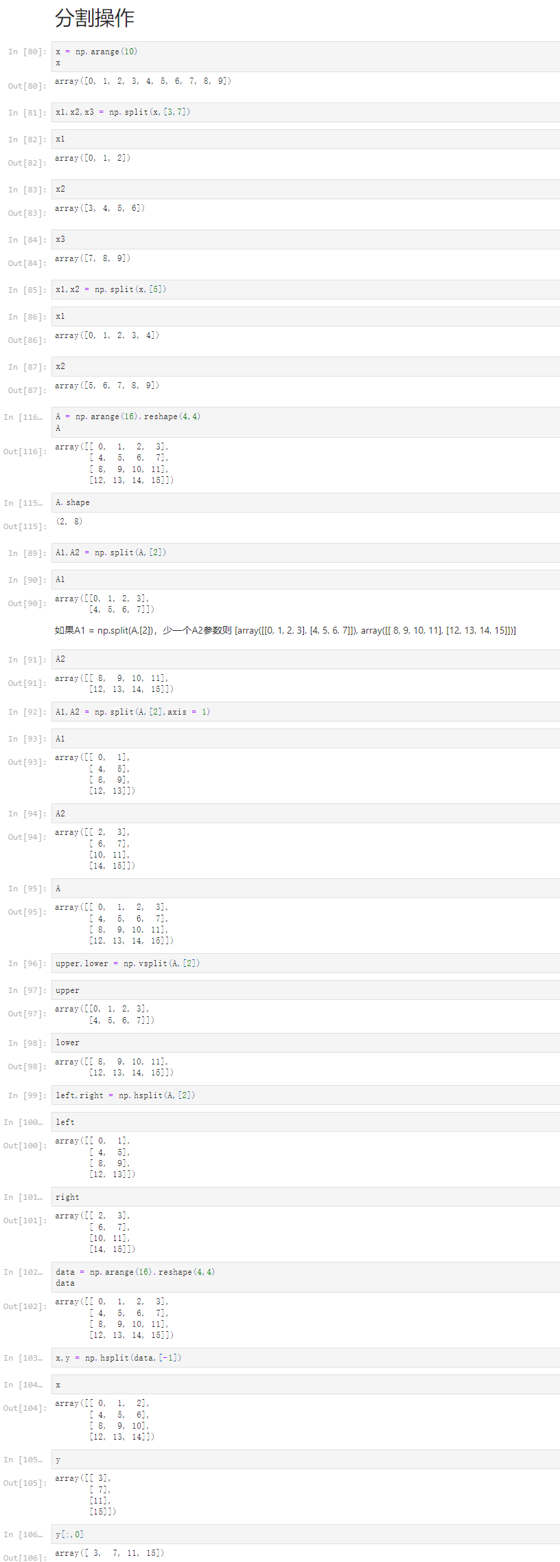
[80]
x = np.arange(10)
x
array([0, 1, 2, 3, 4, 5, 6, 7, 8, 9])
[81]
x1,x2,x3 = np.split(x,[3,7])
[82]
x1
array([0, 1, 2])
[83]
x2
array([3, 4, 5, 6])
[84]
x3
array([7, 8, 9])
[85]
x1,x2 = np.split(x,[5])
[86]
x1
array([0, 1, 2, 3, 4])
[87]
x2
array([5, 6, 7, 8, 9])
[116]
A = np.arange(16).reshape(4,4)
A
array([[ 0, 1, 2, 3],
[ 4, 5, 6, 7],
[ 8, 9, 10, 11],
[12, 13, 14, 15]])
[115]
A.shape
(2, 8)
[89]
A1,A2 = np.split(A,[2])
[90]
A1
array([[0, 1, 2, 3],
[4, 5, 6, 7]])
如果A1 = np.split(A,[2]),少一个A2参数则 [array([[0, 1, 2, 3], [4, 5, 6, 7]]), array([[ 8, 9, 10, 11], [12, 13, 14, 15]])]
[91]
A2
array([[ 8, 9, 10, 11],
[12, 13, 14, 15]])
[92]
A1,A2 = np.split(A,[2],axis = 1)
[93]
A1
array([[ 0, 1],
[ 4, 5],
[ 8, 9],
[12, 13]])
[94]
A2
array([[ 2, 3],
[ 6, 7],
[10, 11],
[14, 15]])
[95]
A
array([[ 0, 1, 2, 3],
[ 4, 5, 6, 7],
[ 8, 9, 10, 11],
[12, 13, 14, 15]])
[96]
upper,lower = np.vsplit(A,[2])
[97]
upper
array([[0, 1, 2, 3],
[4, 5, 6, 7]])
[98]
lower
array([[ 8, 9, 10, 11],
[12, 13, 14, 15]])
[99]
left,right = np.hsplit(A,[2])
[100]
left
array([[ 0, 1],
[ 4, 5],
[ 8, 9],
[12, 13]])
[101]
right
array([[ 2, 3],
[ 6, 7],
[10, 11],
[14, 15]])
[102]
data = np.arange(16).reshape(4,4)
data
array([[ 0, 1, 2, 3],
[ 4, 5, 6, 7],
[ 8, 9, 10, 11],
[12, 13, 14, 15]])
[103]
x,y = np.hsplit(data,[-1])
[104]
x
array([[ 0, 1, 2],
[ 4, 5, 6],
[ 8, 9, 10],
[12, 13, 14]])
[105]
y
array([[ 3],
[ 7],
[11],
[15]])
[106]
y[:,0]
array([ 3, 7, 11, 15])
3-7 Numpy中的矩阵运算
Notbook 示例
Notbook 源码
[1]
n = 10
L = [ i for i in range(n)]
[2]
2 * L
[0, 1, 2, 3, 4, 5, 6, 7, 8, 9, 0, 1, 2, 3, 4, 5, 6, 7, 8, 9]
[3]
A = []
for e in L:
A.append(2*e)
A
[0, 2, 4, 6, 8, 10, 12, 14, 16, 18]
[4]
n = 1000000
L = [ i for i in range(n)]
[5]
%%time
A = []
for e in L:
A.append(2*e)
CPU times: total: 375 ms
Wall time: 449 ms
[6]
%%time
A = [e*2 for e in L]
CPU times: total: 172 ms
Wall time: 209 ms
[7]
import numpy as np
L = np.arange(n)
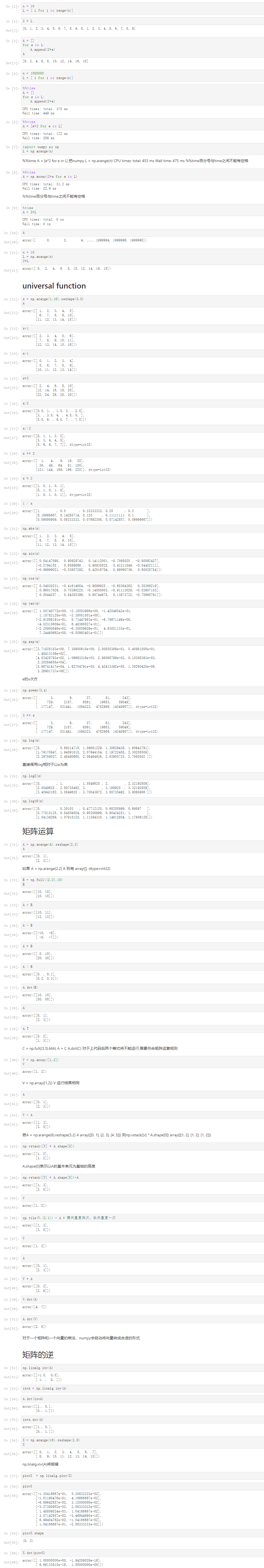
%%time A = [e*2 for e in L] 把numpy L = np.arange(n) CPU times: total: 453 ms Wall time: 475 ms %%time百分号与time之间不能有空格
[8]
%%time
A = np.array(2*e for e in L)
CPU times: total: 31.2 ms
Wall time: 22.9 ms
%%time百分号与time之间不能有空格
[9]
%time
A = 2*L
CPU times: total: 0 ns
Wall time: 0 ns
[10]
A
array([ 0, 2, 4, ..., 1999994, 1999996, 1999998])
[11]
n = 10
L = np.arange(n)
2*L
array([ 0, 2, 4, 6, 8, 10, 12, 14, 16, 18])
universal function
[12]
x = np.arange(1,16).reshape(3,5)
x
array([[ 1, 2, 3, 4, 5],
[ 6, 7, 8, 9, 10],
[11, 12, 13, 14, 15]])
[13]
x+1
array([[ 2, 3, 4, 5, 6],
[ 7, 8, 9, 10, 11],
[12, 13, 14, 15, 16]])
[14]
x-1
array([[ 0, 1, 2, 3, 4],
[ 5, 6, 7, 8, 9],
[10, 11, 12, 13, 14]])
[15]
x*2
array([[ 2, 4, 6, 8, 10],
[12, 14, 16, 18, 20],
[22, 24, 26, 28, 30]])
[16]
x/2
array([[0.5, 1. , 1.5, 2. , 2.5],
[3. , 3.5, 4. , 4.5, 5. ],
[5.5, 6. , 6.5, 7. , 7.5]])
[17]
x//2
array([[0, 1, 1, 2, 2],
[3, 3, 4, 4, 5],
[5, 6, 6, 7, 7]], dtype=int32)
[18]
x ** 2
array([[ 1, 4, 9, 16, 25],
[ 36, 49, 64, 81, 100],
[121, 144, 169, 196, 225]], dtype=int32)
[19]
x % 2
array([[1, 0, 1, 0, 1],
[0, 1, 0, 1, 0],
[1, 0, 1, 0, 1]], dtype=int32)
[20]
1 / x
array([[1. , 0.5 , 0.33333333, 0.25 , 0.2 ],
[0.16666667, 0.14285714, 0.125 , 0.11111111, 0.1 ],
[0.09090909, 0.08333333, 0.07692308, 0.07142857, 0.06666667]])
[21]
np.abs(x)
array([[ 1, 2, 3, 4, 5],
[ 6, 7, 8, 9, 10],
[11, 12, 13, 14, 15]])
[22]
np.sin(x)
array([[ 0.84147098, 0.90929743, 0.14112001, -0.7568025 , -0.95892427],
[-0.2794155 , 0.6569866 , 0.98935825, 0.41211849, -0.54402111],
[-0.99999021, -0.53657292, 0.42016704, 0.99060736, 0.65028784]])
[23]
np.cos(x)
array([[ 0.54030231, -0.41614684, -0.9899925 , -0.65364362, 0.28366219],
[ 0.96017029, 0.75390225, -0.14550003, -0.91113026, -0.83907153],
[ 0.0044257 , 0.84385396, 0.90744678, 0.13673722, -0.75968791]])
[24]
np.tan(x)
array([[ 1.55740772e+00, -2.18503986e+00, -1.42546543e-01,
1.15782128e+00, -3.38051501e+00],
[-2.91006191e-01, 8.71447983e-01, -6.79971146e+00,
-4.52315659e-01, 6.48360827e-01],
[-2.25950846e+02, -6.35859929e-01, 4.63021133e-01,
7.24460662e+00, -8.55993401e-01]])
[25]
np.exp(x)
array([[2.71828183e+00, 7.38905610e+00, 2.00855369e+01, 5.45981500e+01,
1.48413159e+02],
[4.03428793e+02, 1.09663316e+03, 2.98095799e+03, 8.10308393e+03,
2.20264658e+04],
[5.98741417e+04, 1.62754791e+05, 4.42413392e+05, 1.20260428e+06,
3.26901737e+06]])
e的x次方
[26]
np.power(3,x)
array([[ 3, 9, 27, 81, 243],
[ 729, 2187, 6561, 19683, 59049],
[ 177147, 531441, 1594323, 4782969, 14348907]], dtype=int32)
[27]
3 ** x
array([[ 3, 9, 27, 81, 243],
[ 729, 2187, 6561, 19683, 59049],
[ 177147, 531441, 1594323, 4782969, 14348907]], dtype=int32)
[28]
np.log(x)
array([[0. , 0.69314718, 1.09861229, 1.38629436, 1.60943791],
[1.79175947, 1.94591015, 2.07944154, 2.19722458, 2.30258509],
[2.39789527, 2.48490665, 2.56494936, 2.63905733, 2.7080502 ]])
直接调用log相对于以e为底
[29]
np.log2(x)
array([[0. , 1. , 1.5849625 , 2. , 2.32192809],
[2.5849625 , 2.80735492, 3. , 3.169925 , 3.32192809],
[3.45943162, 3.5849625 , 3.70043972, 3.80735492, 3.9068906 ]])
[30]
np.log10(x)
array([[0. , 0.30103 , 0.47712125, 0.60205999, 0.69897 ],
[0.77815125, 0.84509804, 0.90308999, 0.95424251, 1. ],
[1.04139269, 1.07918125, 1.11394335, 1.14612804, 1.17609126]])
矩阵运算
[31]
A = np.arange(4).reshape(2,2)
A
array([[0, 1],
[2, 3]])
如果 A = np.arange(2,2) A 则有 array([], dtype=int32)
[32]
B = np.full((2,2),10)
B
array([[10, 10],
[10, 10]])
[33]
A + B
array([[10, 11],
[12, 13]])
[34]
A - B
array([[-10, -9],
[ -8, -7]])
[35]
A * B
array([[ 0, 10],
[20, 30]])
[36]
A / B
array([[0. , 0.1],
[0.2, 0.3]])
[37]
A.dot(B)
array([[10, 10],
[50, 50]])
[38]
A
array([[0, 1],
[2, 3]])
[39]
A.T
array([[0, 2],
[1, 3]])
C = np.full((3,3),666) A + C A.dot(C) 对于上代码后两个等式将不能运行,需要符合矩阵运算规则
[40]
V = np.array([1,2])
V
array([1, 2])
V = np.array((1,2)) V 运行结果相同
[41]
A
array([[0, 1],
[2, 3]])
[42]
V + A
array([[1, 3],
[3, 5]])
若A = np.arange(6).reshape(3,2) A array([[0, 1], [2, 3], [4, 5]]) 则np.vstack([v] * A.shape[0]) array([[1, 2], [1, 2], [1, 2]])
[43]
np.vstack([V] * A.shape[0])
array([[1, 2],
[1, 2]])
A.shape[0]表示以A的基本单元为基础的高度
[44]
np.vstack([V] * A.shape[0])+A
array([[1, 3],
[3, 5]])
[45]
V
array([1, 2])
[46]
np.tile(V,(2,1)) + A # 横向重复两次,纵向重复一次
array([[1, 3],
[3, 5]])
[47]
V
array([1, 2])
[48]
A
array([[0, 1],
[2, 3]])
[49]
V * A
array([[0, 2],
[2, 6]])
[50]
V.dot(A)
array([4, 7])
[51]
A.dot(V)
array([2, 8])
对于一个矩阵和一个向量的乘法,numpy会自动将向量转成合适的形式
矩阵的逆
[52]
np.linalg.inv(A)
array([[-1.5, 0.5],
[ 1. , 0. ]])
[53]
invA = np.linalg.inv(A)
[54]
A.dot(invA)
array([[1., 0.],
[0., 1.]])
[55]
invA.dot(A)
array([[1., 0.],
[0., 1.]])
[56]
X = np.arange(16).reshape(2,8)
X
array([[ 0, 1, 2, 3, 4, 5, 6, 7],
[ 8, 9, 10, 11, 12, 13, 14, 15]])
np.linalg.inv(A)将报错
[57]
pinvX = np.linalg.pinv(X)
[58]
pinvX
array([[-1.35416667e-01, 5.20833333e-02],
[-1.01190476e-01, 4.16666667e-02],
[-6.69642857e-02, 3.12500000e-02],
[-3.27380952e-02, 2.08333333e-02],
[ 1.48809524e-03, 1.04166667e-02],
[ 3.57142857e-02, -3.46944695e-18],
[ 6.99404762e-02, -1.04166667e-02],
[ 1.04166667e-01, -2.08333333e-02]])
[59]
pinvX.shape
(8, 2)
[60]
X.dot(pinvX)
array([[ 1.00000000e+00, -1.94289029e-16],
[ 6.66133815e-16, 1.00000000e+00]])
3-8 Numpy中的聚合运算and3-9 Numpy中的arg运算
Notbook 示例
Notbook 源码
[1]
import numpy as np
L = np.random.random(100)
[2]
L
array([0.3516844 , 0.65757053, 0.92102817, 0.08232176, 0.29381881,
0.65003014, 0.97971106, 0.5226598 , 0.30206059, 0.08943851,
0.18012353, 0.73187738, 0.21161704, 0.99245898, 0.72893738,
0.81803006, 0.46057643, 0.78305203, 0.21144964, 0.36252883,
0.35272908, 0.25604162, 0.28917731, 0.67740027, 0.90426583,
0.84544952, 0.40110828, 0.04247786, 0.01085229, 0.34014734,
0.70602233, 0.51424636, 0.39786138, 0.36595197, 0.07393888,
0.75163777, 0.45510184, 0.08657692, 0.67168446, 0.88948244,
0.2225157 , 0.2878433 , 0.49303834, 0.81036448, 0.01278707,
0.10601227, 0.89256786, 0.44614657, 0.43688635, 0.79290611,
0.74071001, 0.88761407, 0.28543688, 0.29216674, 0.11519011,
0.73617155, 0.3164547 , 0.37765957, 0.02654595, 0.54816316,
0.81750059, 0.63684799, 0.27424713, 0.1936451 , 0.06800676,
0.8512259 , 0.9296003 , 0.32355494, 0.85864702, 0.59670948,
0.34124613, 0.31258873, 0.64220369, 0.14140289, 0.61121421,
0.05605693, 0.79119813, 0.27604157, 0.74071167, 0.81422001,
0.68846038, 0.56658745, 0.75986556, 0.84020345, 0.93567278,
0.20082763, 0.77921029, 0.22234662, 0.63349144, 0.91545638,
0.44481323, 0.89917595, 0.37389024, 0.68454439, 0.13811925,
0.62240377, 0.96188648, 0.1028726 , 0.11962078, 0.91129131])
[3]
sum (L)
50.26791878652218
[4]
np.sum(L)
50.267918786522195
[5]
big_array = np.random.rand(1000000)
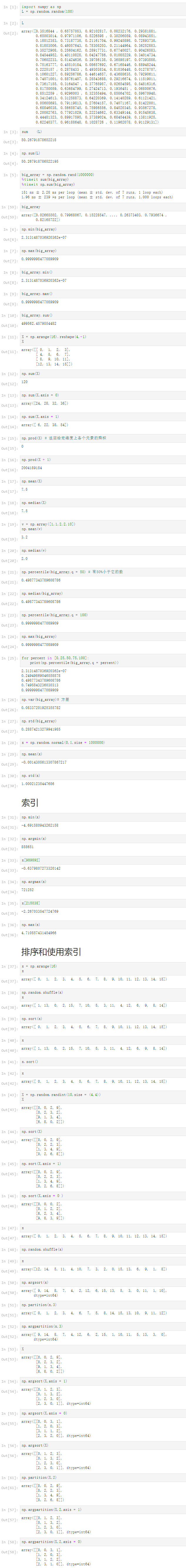
%timeit sum(big_array)
%timeit np.sum(big_array)
151 ms ± 2.28 ms per loop (mean ± std. dev. of 7 runs, 1 loop each)
1.96 ms ± 239 µs per loop (mean ± std. dev. of 7 runs, 1,000 loops each)
[59]
big_array
array([0.02665502, 0.79968067, 0.15228547, ..., 0.26373403, 0.7936674 ,
0.82165722])
[6]
np.min(big_array)
2.3131487036920362e-07
[7]
np.max(big_array)
0.9999998477089909
[8]
big_array.min()
2.3131487036920362e-07
[9]
big_array.max()
0.9999998477089909
[10]
big_array.sum()
499562.4579554482
[11]
X = np.arange(16).reshape(4,-1)
X
array([[ 0, 1, 2, 3],
[ 4, 5, 6, 7],
[ 8, 9, 10, 11],
[12, 13, 14, 15]])
[12]
np.sum(X)
120
[13]
np.sum(X,axis = 0)
array([24, 28, 32, 36])
[14]
np.sum(X,axis = 1)
array([ 6, 22, 38, 54])
[15]
np.prod(X) # 返回给定维度上各个元素的乘积
0
[16]
np.prod(X + 1)
2004189184
[17]
np.mean(X)
7.5
[18]
np.median(X)
7.5
[19]
v = np.array([1,1,2,2,10])
np.mean(v)
3.2
[20]
np.median(v)
2.0
[21]
np.percentile(big_array,q = 50) # 有50%小于它的数
0.49877343789608786
[22]
np.median(big_array)
0.49877343789608786
[23]
np.percentile(big_array,q = 100)
0.9999998477089909
[24]
np.max(big_array)
0.9999998477089909
[25]
for percent in [0,25,50,75,100]:
print(np.percentile(big_array,q = percent))
2.3131487036920362e-07
0.24949869046558878
0.49877343789608786
0.7495843236030313
0.9999998477089909
[26]
np.var(big_array)# 方差
0.08337201925355782
[27]
np.std(big_array)
0.28874213279941985
[28]
x = np.random.normal(0,1,size = 1000000)
[29]
np.mean(x)
-0.0014305613307867217
[30]
np.std(x)
1.00021235447686
索引
[31]
np.min(x)
-4.691580943262158
[32]
np.argmin(x)
858651
[33]
x[989892]
-0.6379807273320142
[34]
np.argmax(x)
721252
[35]
x[215038]
-2.267033547724769
[36]
np.max(x)
4.710557431454966
排序和使用索引
[37]
x = np.arange(16)
x
array([ 0, 1, 2, 3, 4, 5, 6, 7, 8, 9, 10, 11, 12, 13, 14, 15])
[38]
np.random.shuffle(x)
x
array([ 1, 13, 0, 2, 15, 7, 10, 5, 3, 11, 4, 12, 6, 9, 8, 14])
[39]
np.sort(x)
array([ 0, 1, 2, 3, 4, 5, 6, 7, 8, 9, 10, 11, 12, 13, 14, 15])
[40]
x
array([ 1, 13, 0, 2, 15, 7, 10, 5, 3, 11, 4, 12, 6, 9, 8, 14])
[41]
x.sort()
[42]
x
array([ 0, 1, 2, 3, 4, 5, 6, 7, 8, 9, 10, 11, 12, 13, 14, 15])
[43]
X = np.random.randint(10,size = (4,4))
X
array([[0, 0, 2, 9],
[0, 2, 3, 2],
[9, 1, 3, 4],
[6, 8, 0, 2]])
[44]
np.sort(X)
array([[0, 0, 2, 9],
[0, 2, 2, 3],
[1, 3, 4, 9],
[0, 2, 6, 8]])
[45]
np.sort(X,axis = 1)
array([[0, 0, 2, 9],
[0, 2, 2, 3],
[1, 3, 4, 9],
[0, 2, 6, 8]])
[46]
np.sort(X,axis = 0 )
array([[0, 0, 0, 2],
[0, 1, 2, 2],
[6, 2, 3, 4],
[9, 8, 3, 9]])
[47]
x
array([ 0, 1, 2, 3, 4, 5, 6, 7, 8, 9, 10, 11, 12, 13, 14, 15])
[48]
np.random.shuffle(x)
[49]
x
array([12, 14, 5, 11, 4, 10, 7, 3, 2, 0, 15, 13, 6, 9, 1, 8])
[50]
np.argsort(x)
array([ 9, 14, 8, 7, 4, 2, 12, 6, 15, 13, 5, 3, 0, 11, 1, 10],
dtype=int64)
[51]
np.partition(x,3)
array([ 0, 1, 2, 3, 4, 6, 7, 5, 8, 14, 15, 13, 10, 9, 11, 12])
[52]
np.argpartition(x,3)
array([ 9, 14, 8, 7, 4, 12, 6, 2, 15, 1, 10, 11, 5, 13, 3, 0],
dtype=int64)
[53]
X
array([[0, 0, 2, 9],
[0, 2, 3, 2],
[9, 1, 3, 4],
[6, 8, 0, 2]])
[54]
np.argsort(X,axis = 1)
array([[0, 1, 2, 3],
[0, 1, 3, 2],
[1, 2, 3, 0],
[2, 3, 0, 1]], dtype=int64)
[55]
np.argsort(X,axis = 0)
array([[0, 0, 3, 1],
[1, 2, 0, 3],
[3, 1, 1, 2],
[2, 3, 2, 0]], dtype=int64)
[56]
np.argsort(X)
array([[0, 1, 2, 3],
[0, 1, 3, 2],
[1, 2, 3, 0],
[2, 3, 0, 1]], dtype=int64)
[61]
np.partition(X,2)
array([[0, 0, 2, 9],
[0, 2, 2, 3],
[1, 3, 4, 9],
[0, 2, 6, 8]])
[57]
np.argpartition(X,2,axis = 1)
array([[0, 1, 2, 3],
[0, 1, 3, 2],
[1, 2, 3, 0],
[2, 3, 0, 1]], dtype=int64)
[58]
np.argpartition(X,2,axis = 0)
array([[0, 0, 3, 1],
[1, 2, 0, 3],
[3, 1, 2, 2],
[2, 3, 1, 0]], dtype=int64)
3-10 Numpy中的比较和FancyIndexing
Notbook 示例
Notbook 源码
fancy indexing
[1]
import numpy as np
x = np.arange(16)
x
array([ 0, 1, 2, 3, 4, 5, 6, 7, 8, 9, 10, 11, 12, 13, 14, 15])
[2]
x[3]
3
[3]
x[3:9]
array([3, 4, 5, 6, 7, 8])
[4]
x[3:9:2]
array([3, 5, 7])
[5]
[x[3],x[5],x[8]]
[3, 5, 8]
[6]
ind = [3,5,8]
[7]
x[ind]
array([3, 5, 8])
用inw也行,只要对上就OK
[8]
ind = np.array([[0,2],
[1,3]])
x[ind]
array([[0, 2],
[1, 3]])
[9]
X = x.reshape(4,-1)
X
array([[ 0, 1, 2, 3],
[ 4, 5, 6, 7],
[ 8, 9, 10, 11],
[12, 13, 14, 15]])
[10]
row = np.array([0,1,2])
col = np.array([1,2,3])
X[row,col]
array([ 1, 6, 11])
[11]
X[0,col]
array([1, 2, 3])
[12]
X [:2,col]
array([[1, 2, 3],
[5, 6, 7]])
[13]
col = [True ,False,True ,True]
[43]
X = x.reshape(4,-1)
[46]
X[1:3,col]
array([[ 4, 6, 7],
[ 8, 10, 11]])
numpy array的比较
[15]
x
array([ 0, 1, 2, 3, 4, 5, 6, 7, 8, 9, 10, 11, 12, 13, 14, 15])
[16]
x < 3
array([ True, True, True, False, False, False, False, False, False,
False, False, False, False, False, False, False])
[17]
x > 3
array([False, False, False, False, True, True, True, True, True,
True, True, True, True, True, True, True])
[18]
x <= 3
array([ True, True, True, True, False, False, False, False, False,
False, False, False, False, False, False, False])
[19]
x >= 3
array([False, False, False, True, True, True, True, True, True,
True, True, True, True, True, True, True])
[20]
x == 3
array([False, False, False, True, False, False, False, False, False,
False, False, False, False, False, False, False])
[21]
x != 3
array([ True, True, True, False, True, True, True, True, True,
True, True, True, True, True, True, True])
[22]
2 * x == 24 - 4*x
array([False, False, False, False, True, False, False, False, False,
False, False, False, False, False, False, False])
[23]
X
array([[ 0, 1, 2, 3],
[ 4, 5, 6, 7],
[ 8, 9, 10, 11],
[12, 13, 14, 15]])
[24]
X < 6
array([[ True, True, True, True],
[ True, True, False, False],
[False, False, False, False],
[False, False, False, False]])
[25]
x
array([ 0, 1, 2, 3, 4, 5, 6, 7, 8, 9, 10, 11, 12, 13, 14, 15])
[26]
np.sum(x <= 3)
4
[27]
np.count_nonzero(x <= 3)
4
[28]
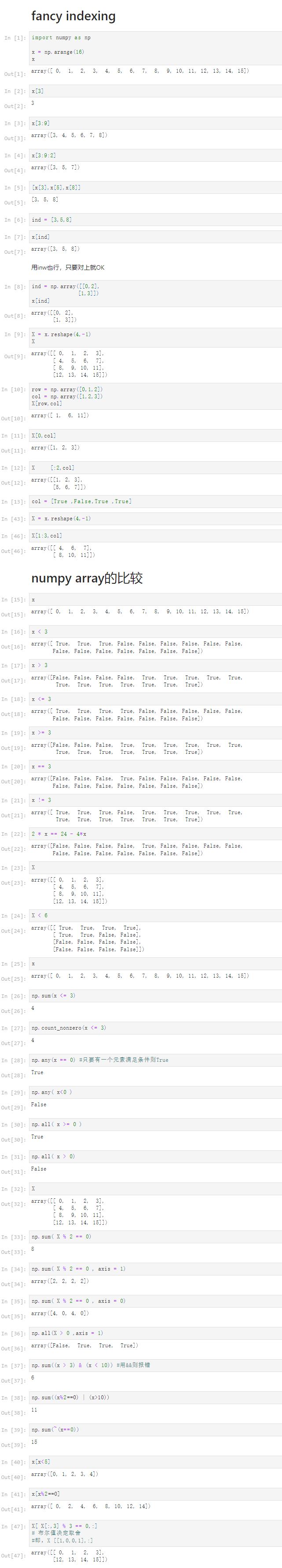
np.any(x == 0) #只要有一个元素满足条件则True
True
[29]
np.any( x<0 )
False
[30]
np.all( x >= 0 )
True
[31]
np.all( x > 0)
False
[32]
X
array([[ 0, 1, 2, 3],
[ 4, 5, 6, 7],
[ 8, 9, 10, 11],
[12, 13, 14, 15]])
[33]
np.sum( X % 2 == 0)
8
[34]
np.sum( X % 2 == 0 , axis = 1)
array([2, 2, 2, 2])
[35]
np.sum( X % 2 == 0 , axis = 0)
array([4, 0, 4, 0])
[36]
np.all(X > 0 ,axis = 1)
array([False, True, True, True])
[37]
np.sum((x > 3) & (x < 10)) #用&&则报错
6
[38]
np.sum((x%2==0) | (x>10))
11
[39]
np.sum(~(x==0))
15
[40]
x[x<5]
array([0, 1, 2, 3, 4])
[41]
x[x%2==0]
array([ 0, 2, 4, 6, 8, 10, 12, 14])
[47]
X[ X[:,3] % 3 == 0,:]
# 布尔值决定取舍
#即,X [[1,0,0,1],:]
array([[ 0, 1, 2, 3],
[12, 13, 14, 15]])
3-11 Matplotlib数据可视化基础
Notbook 示例
Notbook 源码
[1]
#import matplotlib as mpl
[2]
import matplotlib.pyplot as plt
[3]
import numpy as np
[4]
x = np.linspace(0,10,100)
[5]
x
array([ 0. , 0.1010101 , 0.2020202 , 0.3030303 , 0.4040404 ,
0.50505051, 0.60606061, 0.70707071, 0.80808081, 0.90909091,
1.01010101, 1.11111111, 1.21212121, 1.31313131, 1.41414141,
1.51515152, 1.61616162, 1.71717172, 1.81818182, 1.91919192,
2.02020202, 2.12121212, 2.22222222, 2.32323232, 2.42424242,
2.52525253, 2.62626263, 2.72727273, 2.82828283, 2.92929293,
3.03030303, 3.13131313, 3.23232323, 3.33333333, 3.43434343,
3.53535354, 3.63636364, 3.73737374, 3.83838384, 3.93939394,
4.04040404, 4.14141414, 4.24242424, 4.34343434, 4.44444444,
4.54545455, 4.64646465, 4.74747475, 4.84848485, 4.94949495,
5.05050505, 5.15151515, 5.25252525, 5.35353535, 5.45454545,
5.55555556, 5.65656566, 5.75757576, 5.85858586, 5.95959596,
6.06060606, 6.16161616, 6.26262626, 6.36363636, 6.46464646,
6.56565657, 6.66666667, 6.76767677, 6.86868687, 6.96969697,
7.07070707, 7.17171717, 7.27272727, 7.37373737, 7.47474747,
7.57575758, 7.67676768, 7.77777778, 7.87878788, 7.97979798,
8.08080808, 8.18181818, 8.28282828, 8.38383838, 8.48484848,
8.58585859, 8.68686869, 8.78787879, 8.88888889, 8.98989899,
9.09090909, 9.19191919, 9.29292929, 9.39393939, 9.49494949,
9.5959596 , 9.6969697 , 9.7979798 , 9.8989899 , 10. ])
[6]
y = np.sin(x)
[7]
y
array([ 0. , 0.10083842, 0.20064886, 0.2984138 , 0.39313661,
0.48385164, 0.56963411, 0.64960951, 0.72296256, 0.78894546,
0.84688556, 0.8961922 , 0.93636273, 0.96698762, 0.98775469,
0.99845223, 0.99897117, 0.98930624, 0.96955595, 0.93992165,
0.90070545, 0.85230712, 0.79522006, 0.73002623, 0.65739025,
0.57805259, 0.49282204, 0.40256749, 0.30820902, 0.21070855,
0.11106004, 0.01027934, -0.09060615, -0.19056796, -0.28858706,
-0.38366419, -0.47483011, -0.56115544, -0.64176014, -0.7158225 ,
-0.7825875 , -0.84137452, -0.89158426, -0.93270486, -0.96431712,
-0.98609877, -0.99782778, -0.99938456, -0.99075324, -0.97202182,
-0.94338126, -0.90512352, -0.85763861, -0.80141062, -0.73701276,
-0.66510151, -0.58640998, -0.50174037, -0.41195583, -0.31797166,
-0.22074597, -0.12126992, -0.0205576 , 0.0803643 , 0.18046693,
0.27872982, 0.37415123, 0.46575841, 0.55261747, 0.63384295,
0.7086068 , 0.77614685, 0.83577457, 0.8868821 , 0.92894843,
0.96154471, 0.98433866, 0.99709789, 0.99969234, 0.99209556,
0.97438499, 0.94674118, 0.90944594, 0.86287948, 0.8075165 ,
0.74392141, 0.6727425 , 0.59470541, 0.51060568, 0.42130064,
0.32770071, 0.23076008, 0.13146699, 0.03083368, -0.07011396,
-0.17034683, -0.26884313, -0.36459873, -0.45663749, -0.54402111])
[8]
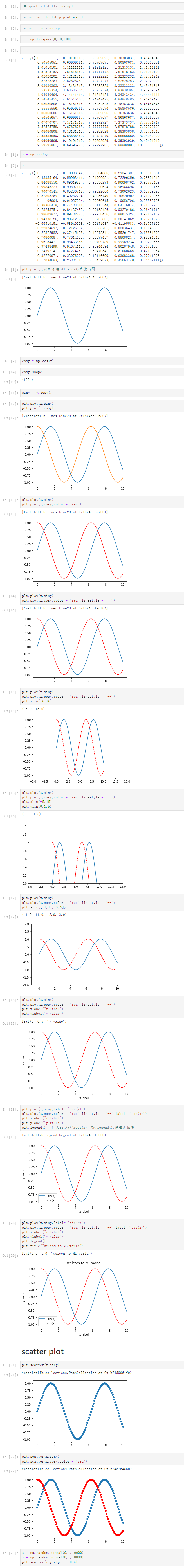
plt.plot(x,y)# 不用plt.show()直接出图
[<matplotlib.lines.Line2D at 0x1b74c435760>]
[9]
cosy = np.cos(x)
[10]
cosy.shape
(100,)
[11]
siny = y.copy()
[12]
plt.plot(x,siny)
plt.plot(x,cosy)
[<matplotlib.lines.Line2D at 0x1b74c539b80>]
[13]
plt.plot(x,siny)
plt.plot(x,cosy,color = 'red')
[<matplotlib.lines.Line2D at 0x1b74c5b2700>]
[14]
plt.plot(x,siny)
plt.plot(x,cosy,color = 'red',linestyle = '--')
[<matplotlib.lines.Line2D at 0x1b74c61adf0>]
[15]
plt.plot(x,siny)
plt.plot(x,cosy,color = 'red',linestyle = '--')
plt.xlim(-5,15)
(-5.0, 15.0)
[16]
plt.plot(x,siny)
plt.plot(x,cosy,color = 'red',linestyle = '--')
plt.xlim(-5,15)
plt.ylim(0,1.5)
(0.0, 1.5)
[17]
plt.plot(x,siny)
plt.plot(x,cosy,color = 'red',linestyle = '--')
plt.axis([-1,11,-2,2])
(-1.0, 11.0, -2.0, 2.0)
[18]
plt.plot(x,siny)
plt.plot(x,cosy,color = 'red',linestyle = '--')
plt.xlabel("x label")
plt.ylabel('y value')
Text(0, 0.5, 'y value')
[19]
plt.plot(x,siny,label= 'sin(x)')
plt.plot(x,cosy,color = 'red',linestyle = '--',label= 'cos(x)')
plt.xlabel("x label")
plt.ylabel('y value')
plt.legend() # 无sin(x)与cos(x)下标,legend(),需要加括号
<matplotlib.legend.Legend at 0x1b74d815bb0>
[20]
plt.plot(x,siny,label= 'sin(x)')
plt.plot(x,cosy,color = 'red',linestyle = '--',label= 'cos(x)')
plt.xlabel("x label")
plt.ylabel('y value')
plt.legend()
plt.title("welcom to ML world")
Text(0.5, 1.0, 'welcom to ML world')
scatter plot
[21]
plt.scatter(x,siny)
<matplotlib.collections.PathCollection at 0x1b74d9064f0>
[22]
plt.scatter(x,siny)
plt.scatter(x,cosy,color = "red")
<matplotlib.collections.PathCollection at 0x1b74c764a60>
[23]
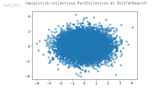
x = np.random.normal(0,1,10000)
y = np.random.normal(0,1,10000)
plt.scatter(x,y,alpha = 0.5)
<matplotlib.collections.PathCollection at 0x1b74c6eac10>
3-12 数据加载和简单的数据探索
Notbook 示例

Notbook 源码
[1]
import numpy as np
[2]
# import matplotlib as mpl
import matplotlib.pyplot as plt
[3]
from sklearn import datasets
[4]
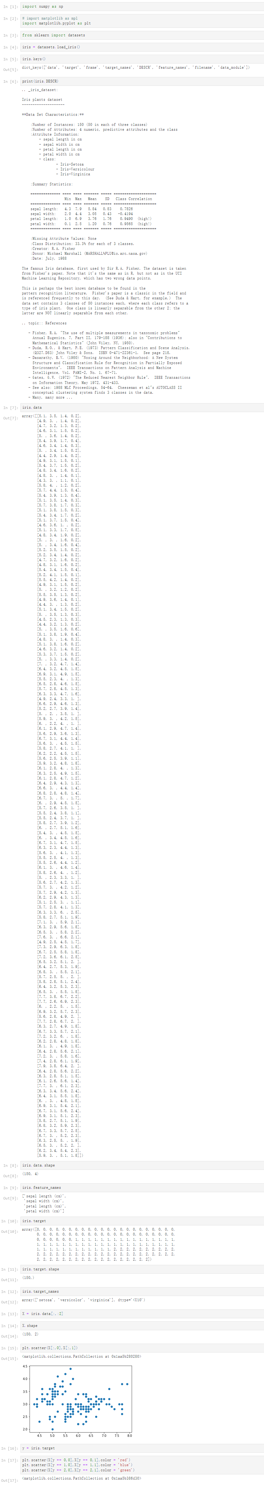
iris = datasets.load_iris()
[5]
iris.keys()
dict_keys(['data', 'target', 'frame', 'target_names', 'DESCR', 'feature_names', 'filename', 'data_module'])
[6]
print(iris.DESCR)
.. _iris_dataset:
Iris plants dataset
--------------------
**Data Set Characteristics:**
:Number of Instances: 150 (50 in each of three classes)
:Number of Attributes: 4 numeric, predictive attributes and the class
:Attribute Information:
- sepal length in cm
- sepal width in cm
- petal length in cm
- petal width in cm
- class:
- Iris-Setosa
- Iris-Versicolour
- Iris-Virginica
:Summary Statistics:
============== ==== ==== ======= ===== ====================
Min Max Mean SD Class Correlation
============== ==== ==== ======= ===== ====================
sepal length: 4.3 7.9 5.84 0.83 0.7826
sepal width: 2.0 4.4 3.05 0.43 -0.4194
petal length: 1.0 6.9 3.76 1.76 0.9490 (high!)
petal width: 0.1 2.5 1.20 0.76 0.9565 (high!)
============== ==== ==== ======= ===== ====================
:Missing Attribute Values: None
:Class Distribution: 33.3% for each of 3 classes.
:Creator: R.A. Fisher
:Donor: Michael Marshall (MARSHALL%[email protected])
:Date: July, 1988
The famous Iris database, first used by Sir R.A. Fisher. The dataset is taken
from Fisher's paper. Note that it's the same as in R, but not as in the UCI
Machine Learning Repository, which has two wrong data points.
This is perhaps the best known database to be found in the
pattern recognition literature. Fisher's paper is a classic in the field and
is referenced frequently to this day. (See Duda & Hart, for example.) The
data set contains 3 classes of 50 instances each, where each class refers to a
type of iris plant. One class is linearly separable from the other 2; the
latter are NOT linearly separable from each other.
.. topic:: References
- Fisher, R.A. "The use of multiple measurements in taxonomic problems"
Annual Eugenics, 7, Part II, 179-188 (1936); also in "Contributions to
Mathematical Statistics" (John Wiley, NY, 1950).
- Duda, R.O., & Hart, P.E. (1973) Pattern Classification and Scene Analysis.
(Q327.D83) John Wiley & Sons. ISBN 0-471-22361-1. See page 218.
- Dasarathy, B.V. (1980) "Nosing Around the Neighborhood: A New System
Structure and Classification Rule for Recognition in Partially Exposed
Environments". IEEE Transactions on Pattern Analysis and Machine
Intelligence, Vol. PAMI-2, No. 1, 67-71.
- Gates, G.W. (1972) "The Reduced Nearest Neighbor Rule". IEEE Transactions
on Information Theory, May 1972, 431-433.
- See also: 1988 MLC Proceedings, 54-64. Cheeseman et al"s AUTOCLASS II
conceptual clustering system finds 3 classes in the data.
- Many, many more ...
[7]
iris.data
array([[5.1, 3.5, 1.4, 0.2],
[4.9, 3. , 1.4, 0.2],
[4.7, 3.2, 1.3, 0.2],
[4.6, 3.1, 1.5, 0.2],
[5. , 3.6, 1.4, 0.2],
[5.4, 3.9, 1.7, 0.4],
[4.6, 3.4, 1.4, 0.3],
[5. , 3.4, 1.5, 0.2],
[4.4, 2.9, 1.4, 0.2],
[4.9, 3.1, 1.5, 0.1],
[5.4, 3.7, 1.5, 0.2],
[4.8, 3.4, 1.6, 0.2],
[4.8, 3. , 1.4, 0.1],
[4.3, 3. , 1.1, 0.1],
[5.8, 4. , 1.2, 0.2],
[5.7, 4.4, 1.5, 0.4],
[5.4, 3.9, 1.3, 0.4],
[5.1, 3.5, 1.4, 0.3],
[5.7, 3.8, 1.7, 0.3],
[5.1, 3.8, 1.5, 0.3],
[5.4, 3.4, 1.7, 0.2],
[5.1, 3.7, 1.5, 0.4],
[4.6, 3.6, 1. , 0.2],
[5.1, 3.3, 1.7, 0.5],
[4.8, 3.4, 1.9, 0.2],
[5. , 3. , 1.6, 0.2],
[5. , 3.4, 1.6, 0.4],
[5.2, 3.5, 1.5, 0.2],
[5.2, 3.4, 1.4, 0.2],
[4.7, 3.2, 1.6, 0.2],
[4.8, 3.1, 1.6, 0.2],
[5.4, 3.4, 1.5, 0.4],
[5.2, 4.1, 1.5, 0.1],
[5.5, 4.2, 1.4, 0.2],
[4.9, 3.1, 1.5, 0.2],
[5. , 3.2, 1.2, 0.2],
[5.5, 3.5, 1.3, 0.2],
[4.9, 3.6, 1.4, 0.1],
[4.4, 3. , 1.3, 0.2],
[5.1, 3.4, 1.5, 0.2],
[5. , 3.5, 1.3, 0.3],
[4.5, 2.3, 1.3, 0.3],
[4.4, 3.2, 1.3, 0.2],
[5. , 3.5, 1.6, 0.6],
[5.1, 3.8, 1.9, 0.4],
[4.8, 3. , 1.4, 0.3],
[5.1, 3.8, 1.6, 0.2],
[4.6, 3.2, 1.4, 0.2],
[5.3, 3.7, 1.5, 0.2],
[5. , 3.3, 1.4, 0.2],
[7. , 3.2, 4.7, 1.4],
[6.4, 3.2, 4.5, 1.5],
[6.9, 3.1, 4.9, 1.5],
[5.5, 2.3, 4. , 1.3],
[6.5, 2.8, 4.6, 1.5],
[5.7, 2.8, 4.5, 1.3],
[6.3, 3.3, 4.7, 1.6],
[4.9, 2.4, 3.3, 1. ],
[6.6, 2.9, 4.6, 1.3],
[5.2, 2.7, 3.9, 1.4],
[5. , 2. , 3.5, 1. ],
[5.9, 3. , 4.2, 1.5],
[6. , 2.2, 4. , 1. ],
[6.1, 2.9, 4.7, 1.4],
[5.6, 2.9, 3.6, 1.3],
[6.7, 3.1, 4.4, 1.4],
[5.6, 3. , 4.5, 1.5],
[5.8, 2.7, 4.1, 1. ],
[6.2, 2.2, 4.5, 1.5],
[5.6, 2.5, 3.9, 1.1],
[5.9, 3.2, 4.8, 1.8],
[6.1, 2.8, 4. , 1.3],
[6.3, 2.5, 4.9, 1.5],
[6.1, 2.8, 4.7, 1.2],
[6.4, 2.9, 4.3, 1.3],
[6.6, 3. , 4.4, 1.4],
[6.8, 2.8, 4.8, 1.4],
[6.7, 3. , 5. , 1.7],
[6. , 2.9, 4.5, 1.5],
[5.7, 2.6, 3.5, 1. ],
[5.5, 2.4, 3.8, 1.1],
[5.5, 2.4, 3.7, 1. ],
[5.8, 2.7, 3.9, 1.2],
[6. , 2.7, 5.1, 1.6],
[5.4, 3. , 4.5, 1.5],
[6. , 3.4, 4.5, 1.6],
[6.7, 3.1, 4.7, 1.5],
[6.3, 2.3, 4.4, 1.3],
[5.6, 3. , 4.1, 1.3],
[5.5, 2.5, 4. , 1.3],
[5.5, 2.6, 4.4, 1.2],
[6.1, 3. , 4.6, 1.4],
[5.8, 2.6, 4. , 1.2],
[5. , 2.3, 3.3, 1. ],
[5.6, 2.7, 4.2, 1.3],
[5.7, 3. , 4.2, 1.2],
[5.7, 2.9, 4.2, 1.3],
[6.2, 2.9, 4.3, 1.3],
[5.1, 2.5, 3. , 1.1],
[5.7, 2.8, 4.1, 1.3],
[6.3, 3.3, 6. , 2.5],
[5.8, 2.7, 5.1, 1.9],
[7.1, 3. , 5.9, 2.1],
[6.3, 2.9, 5.6, 1.8],
[6.5, 3. , 5.8, 2.2],
[7.6, 3. , 6.6, 2.1],
[4.9, 2.5, 4.5, 1.7],
[7.3, 2.9, 6.3, 1.8],
[6.7, 2.5, 5.8, 1.8],
[7.2, 3.6, 6.1, 2.5],
[6.5, 3.2, 5.1, 2. ],
[6.4, 2.7, 5.3, 1.9],
[6.8, 3. , 5.5, 2.1],
[5.7, 2.5, 5. , 2. ],
[5.8, 2.8, 5.1, 2.4],
[6.4, 3.2, 5.3, 2.3],
[6.5, 3. , 5.5, 1.8],
[7.7, 3.8, 6.7, 2.2],
[7.7, 2.6, 6.9, 2.3],
[6. , 2.2, 5. , 1.5],
[6.9, 3.2, 5.7, 2.3],
[5.6, 2.8, 4.9, 2. ],
[7.7, 2.8, 6.7, 2. ],
[6.3, 2.7, 4.9, 1.8],
[6.7, 3.3, 5.7, 2.1],
[7.2, 3.2, 6. , 1.8],
[6.2, 2.8, 4.8, 1.8],
[6.1, 3. , 4.9, 1.8],
[6.4, 2.8, 5.6, 2.1],
[7.2, 3. , 5.8, 1.6],
[7.4, 2.8, 6.1, 1.9],
[7.9, 3.8, 6.4, 2. ],
[6.4, 2.8, 5.6, 2.2],
[6.3, 2.8, 5.1, 1.5],
[6.1, 2.6, 5.6, 1.4],
[7.7, 3. , 6.1, 2.3],
[6.3, 3.4, 5.6, 2.4],
[6.4, 3.1, 5.5, 1.8],
[6. , 3. , 4.8, 1.8],
[6.9, 3.1, 5.4, 2.1],
[6.7, 3.1, 5.6, 2.4],
[6.9, 3.1, 5.1, 2.3],
[5.8, 2.7, 5.1, 1.9],
[6.8, 3.2, 5.9, 2.3],
[6.7, 3.3, 5.7, 2.5],
[6.7, 3. , 5.2, 2.3],
[6.3, 2.5, 5. , 1.9],
[6.5, 3. , 5.2, 2. ],
[6.2, 3.4, 5.4, 2.3],
[5.9, 3. , 5.1, 1.8]])
[8]
iris.data.shape
(150, 4)
[9]
iris.feature_names
['sepal length (cm)',
'sepal width (cm)',
'petal length (cm)',
'petal width (cm)']
[10]
iris.target
array([0, 0, 0, 0, 0, 0, 0, 0, 0, 0, 0, 0, 0, 0, 0, 0, 0, 0, 0, 0, 0, 0,
0, 0, 0, 0, 0, 0, 0, 0, 0, 0, 0, 0, 0, 0, 0, 0, 0, 0, 0, 0, 0, 0,
0, 0, 0, 0, 0, 0, 1, 1, 1, 1, 1, 1, 1, 1, 1, 1, 1, 1, 1, 1, 1, 1,
1, 1, 1, 1, 1, 1, 1, 1, 1, 1, 1, 1, 1, 1, 1, 1, 1, 1, 1, 1, 1, 1,
1, 1, 1, 1, 1, 1, 1, 1, 1, 1, 1, 1, 2, 2, 2, 2, 2, 2, 2, 2, 2, 2,
2, 2, 2, 2, 2, 2, 2, 2, 2, 2, 2, 2, 2, 2, 2, 2, 2, 2, 2, 2, 2, 2,
2, 2, 2, 2, 2, 2, 2, 2, 2, 2, 2, 2, 2, 2, 2, 2, 2, 2])
[11]
iris.target.shape
(150,)
[12]
iris.target_names
array(['setosa', 'versicolor', 'virginica'], dtype='<U10')
[13]
X = iris.data[:,:2]
[14]
X.shape
(150, 2)
[15]
plt.scatter(X[:,0],X[:,1])
<matplotlib.collections.PathCollection at 0x1aa5b280280>
[16]
y = iris.target
[17]
plt.scatter(X[y == 0,0],X[y == 0,1],color = 'red')
plt.scatter(X[y == 1,0],X[y == 1,1],color = 'blue')
plt.scatter(X[y == 2,0],X[y == 2,1],color = 'green')
<matplotlib.collections.PathCollection at 0x1aa5b386d30>
[18]
plt.scatter(X[y == 0,0],X[y == 0,1],color = 'red',marker='o')
plt.scatter(X[y == 1,0],X[y == 1,1],color = 'blue',marker='+')
plt.scatter(X[y == 2,0],X[y == 2,1],color = 'green',marker='x')
<matplotlib.collections.PathCollection at 0x1aa5b4089d0>
[19]
X = iris.data[:,2:]
[20]
plt.scatter(X[y == 0,0],X[y == 0,1],color = 'red',marker='o')
plt.scatter(X[y == 1,0],X[y == 1,1],color = 'blue',marker='+')
plt.scatter(X[y == 2,0],X[y == 2,1],color = 'green',marker='x')
<matplotlib.collections.PathCollection at 0x1aa5b46f640>