前言:这是我机器学习的课程设计,实现的是在YOLOv5目标检测的基础上增加语义分割头,然后在Cityscapes数据集上进行训练,代码参考的是TomMo23链接如下:TomMao23/multiyolov5: joint detection and semantic segmentation, based on ultralytics/yolov5, (github.com)在此基础上,增加了车道检测并计算车道的曲率半径,同时计算车辆偏离车道中心的距离,也可计算出识别出的车辆距离本车辆的距离。项目主要分为两大块内容:用传统方法即opencv通过图像矫正、二值化、图像变换对二值化图像进行梯度阈值过滤和颜色阈值过滤然后进行二次函数拟合识别出车道线;第二块内容就是YOLOv5识别各种车辆和交通灯。
一、车道检测
1.1.相机矫正
由于拍摄得到的图像可能存在畸变,或者不正的情况,所以在做后面的步骤前需要进行相机矫正,这边使用了opencv中的calibrateCamera()方法拍摄相当数量不同角度和品质的棋盘格图像来得到相机标定矩阵。
def get_obj_img_points(images,grid=(9,6)):
    object_points=[]
    img_points = []
    for img in images:
        #生成object points
        object_point = np.zeros( (grid[0]*grid[1],3),np.float32 )
        object_point[:,:2]= np.mgrid[0:grid[0],0:grid[1]].T.reshape(-1,2)
        #得到灰度图片
        gray = cv2.cvtColor(img,cv2.COLOR_BGR2GRAY)
        #得到图片的image points
        ret, corners = cv2.findChessboardCorners(gray, grid, None)
        if ret:
            object_points.append(object_point)
            img_points.append(corners)
    return object_points,img_points
然后把上述的参数传入cv的calibrateCamera() 方法中就可以计算出相机校正矩阵(camera calibration matrix)和失真系数(distortion coefficients),再使用 cv2.undistort()方法就可得到校正图片。
def cal_undistort(img, objpoints, imgpoints):
    ret, mtx, dist, rvecs, tvecs = cv2.calibrateCamera(objpoints, imgpoints, img.shape[1::-1], None, None)
    dst = cv2.undistort(img, mtx, dist, None, mtx)
    return dst
1.2阈值过滤
在经过相机矫正后继续经过阈值过滤可以得到清晰捕捉车道线的二进制图,经过几种阈值处理方法最后决定同时使用梯度阈值和颜色阈值过滤的方法。采用水平梯度变化,通过测试发现方向阈值在35到100区间过滤得出的二进制图可以捕捉较为清晰的车道线。实现代码如下:
def abs_sobel_thresh(img, orient='x', thresh_min=0, thresh_max=255):
    # Convert to grayscale
    gray = cv2.cvtColor(img, cv2.COLOR_RGB2GRAY)
    # Apply x or y gradient with the OpenCV Sobel() function
    # and take the absolute value
    if orient == 'x':
        abs_sobel = np.absolute(cv2.Sobel(gray, cv2.CV_64F, 1, 0))
    if orient == 'y':
        abs_sobel = np.absolute(cv2.Sobel(gray, cv2.CV_64F, 0, 1))
    # Rescale back to 8 bit integer
    scaled_sobel = np.uint8(255 * abs_sobel / np.max(abs_sobel))
    # Create a copy and apply the threshold
    binary_output = np.zeros_like(scaled_sobel)
    # Here I'm using inclusive (>=, <=) thresholds, but exclusive is ok too
    binary_output[(scaled_sobel >= thresh_min) & (scaled_sobel <= thresh_max)] = 1

    # Return the result
    return binary_output

def hls_select(img, channel='s', thresh=(0, 255)):
    hls = cv2.cvtColor(img, cv2.COLOR_RGB2HLS)
    if channel == 'h':
        channel = hls[:, :, 0]
    elif channel == 'l':
        channel = hls[:, :, 1]
    else:
        channel = hls[:, :, 2]
    binary_output = np.zeros_like(channel)
    binary_output[(channel > thresh[0]) & (channel <= thresh[1])] = 1
    return binary_output
1.3车道检测
首先要定位车道线的基点(图片最下方车道出现的x轴坐标),由于车道线在的像素都集中在x轴一定范围内,因此把图片一分为二,则左右两边的在x轴上的像素分布峰值非常有可能就是车道线基点。
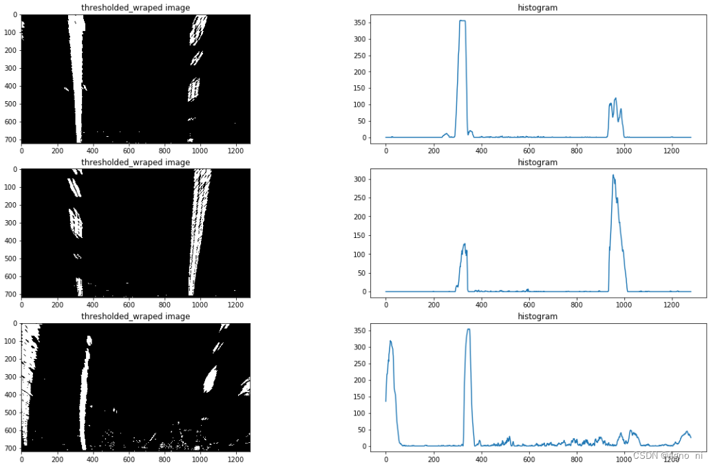
沿x轴对图像进行采样,当白色像素点急剧变化的地方就认为是车道线所在的位置。
def find_line_by_previous(binary_warped, left_fit, right_fit):
    nonzero = binary_warped.nonzero()
    nonzeroy = np.array(nonzero[0])
    nonzerox = np.array(nonzero[1])
    margin = 100
    left_lane_inds = ((nonzerox > (left_fit[0] * (nonzeroy ** 2) + left_fit[1] * nonzeroy +
                                   left_fit[2] - margin)) & (nonzerox < (left_fit[0] * (nonzeroy ** 2) +
                                                                         left_fit[1] * nonzeroy + left_fit[
                                                                             2] + margin)))

    right_lane_inds = ((nonzerox > (right_fit[0] * (nonzeroy ** 2) + right_fit[1] * nonzeroy +
                                    right_fit[2] - margin)) & (nonzerox < (right_fit[0] * (nonzeroy ** 2) +
                                                                           right_fit[1] * nonzeroy + right_fit[
                                                                               2] + margin)))

    # Again, extract left and right line pixel positions
    leftx = nonzerox[left_lane_inds]
    lefty = nonzeroy[left_lane_inds]
    rightx = nonzerox[right_lane_inds]
    righty = nonzeroy[right_lane_inds]
    # Fit a second order polynomial to each
    left_fit = np.polyfit(lefty, leftx, 2)
    right_fit = np.polyfit(righty, rightx, 2)
    return left_fit, right_fit, left_lane_inds, right_lane_inds
还可以得到一个带x轴索引的y方向像素均值元组,可以将其作为拟合曲线的x,y输入numpy的polyfit()方法产生拟合曲线。 然后确定每像素与在世界坐标中距离的对应关系,基于此对应关系和上述产生的拟合曲线结合生成新的拟合曲线,此拟合曲线反应的是显示车道线,再代入公式 然后计算偏离中心位置的距离,由于前面所有对于图像处理的过程关系,此处可以近似将图像二值图像中心的x值,将其与每像素与在世界坐标中距离的对应关系相乘,此值与未经过对应关系转换的拟合曲线的最后一个值,经过对应关系转换的差值就是偏离车道中心的实际距离。 使用逆变形矩阵把鸟瞰二进制图检测的车道镶嵌回原图,并高亮车道区域,使用opencv的putText()方法处理原图展示车道曲率及车辆相对车道中心位置信息
def draw_area(undist, binary_warped, Minv, left_fit, right_fit):
    # Generate x and y values for plotting
    ploty = np.linspace(0, binary_warped.shape[0] - 1, binary_warped.shape[0])
    left_fitx = left_fit[0] * ploty ** 2 + left_fit[1] * ploty + left_fit[2]
    right_fitx = right_fit[0] * ploty ** 2 + right_fit[1] * ploty + right_fit[2]
    # Create an image to draw the lines on
    warp_zero = np.zeros_like(binary_warped).astype(np.uint8)
    color_warp = np.dstack((warp_zero, warp_zero, warp_zero))

    # Recast the x and y points into usable format for cv2.fillPoly()
    pts_left = np.array([np.transpose(np.vstack([left_fitx, ploty]))])
    pts_right = np.array([np.flipud(np.transpose(np.vstack([right_fitx, ploty])))])
    pts = np.hstack((pts_left, pts_right))

    # Draw the lane onto the warped blank image
    cv2.fillPoly(color_warp, np.int_([pts]), (0, 255, 0))

    # Warp the blank back to original image space using inverse perspective matrix (Minv)
    newwarp = cv2.warpPerspective(color_warp, Minv, (undist.shape[1], undist.shape[0]))
    # Combine the result with the original image
    result = cv2.addWeighted(undist, 1, newwarp, 0.3, 0)
    return result


#   计算曲率和半径
def calculate_curv_and_pos(binary_warped, left_fit, right_fit):
    # Define y-value where we want radius of curvature
    ploty = np.linspace(0, binary_warped.shape[0] - 1, binary_warped.shape[0])
    leftx = left_fit[0] * ploty ** 2 + left_fit[1] * ploty + left_fit[2]
    rightx = right_fit[0] * ploty ** 2 + right_fit[1] * ploty + right_fit[2]
    # Define conversions in x and y from pixels space to meters
    ym_per_pix = 30 / 720  # meters per pixel in y dimension
    xm_per_pix = 3.7 / 700  # meters per pixel in x dimension
    y_eval = np.max(ploty)
    # Fit new polynomials to x,y in world space
    left_fit_cr = np.polyfit(ploty * ym_per_pix, leftx * xm_per_pix, 2)
    right_fit_cr = np.polyfit(ploty * ym_per_pix, rightx * xm_per_pix, 2)
    # Calculate the new radii of curvature
    left_curverad = ((1 + (2 * left_fit_cr[0] * y_eval * ym_per_pix + left_fit_cr[1]) ** 2) ** 1.5) / np.absolute(
        2 * left_fit_cr[0])
    right_curverad = ((1 + (2 * right_fit_cr[0] * y_eval * ym_per_pix + right_fit_cr[1]) ** 2) ** 1.5) / np.absolute(
        2 * right_fit_cr[0])

    curvature = ((left_curverad + right_curverad) / 2)
    # print(curvature)
    lane_width = np.absolute(leftx[719] - rightx[719])
    lane_xm_per_pix = 3.7 / lane_width
    veh_pos = (((leftx[719] + rightx[719]) * lane_xm_per_pix) / 2.)
    cen_pos = ((binary_warped.shape[1] * lane_xm_per_pix) / 2.)
    distance_from_center = cen_pos - veh_pos
    return curvature, distance_from_center


def calculate_position(bbox, transform_matrix, warped_size, pix_per_meter):
    if len(bbox) == 0:
        print("nothing")
    else:
        pos = np.array((bbox[1] / 2 + bbox[3] / 2, bbox[2])).reshape(1, 1, -1)
        dst = cv2.perspectiveTransform(pos, transform_matrix).reshape(-1, 1)
        return np.array((warped_size[1] - dst[1]) / pix_per_meter[1])

def draw_values(img, curvature, distance_from_center):
    font = cv2.FONT_HERSHEY_SIMPLEX
    radius_text = "Radius of Curvature: %sm" % (round(curvature))

    if distance_from_center > 0:
        pos_flag = 'right'
    else:
        pos_flag = 'left'

    cv2.putText(img, radius_text, (100, 100), font, 1, (255, 255, 255), 2)
    center_text = "Vehicle is %.3fm %s of center" % (abs(distance_from_center), pos_flag)
    cv2.putText(img, center_text, (100, 150), font, 1, (255, 255, 255), 2)
    return img
二、YOLOV5
YOLOv5是一种单阶段目标检测算法,该算法在YOLOv3的基础上添加了一些新的改进思路:使用Pytorch框架更容易投入生产,整合了计算机视觉领域的State-of-the-art等算法
由于训练需要的图片数据庞大,所以训练集图片我们使用的是国外数据集Cityscapes,即城市景观数据集,该数据集拥有5000张在城市环境中驾驶场景的图像。在本次训练中我们用2975张图片作为训练集,500张作为验证集,1525张图片作为测试集。
本次实验训练的模型在Cityscapes语义分割数据集和由Cityscapes实例分割标签转换来的目标检测数据集上同时训练,这样就可以在进行目标检测的同时同时进行语义分割。
这部分的代码和配置过程TomMo的readme里面已经写得很清楚了,我这边就不在赘述了,大家按他的教程来一般就可以训练自己的模型出来。
我最后就放一下我最后的效果吧~
YOLOv5自动驾驶