文章目录

将Hough Line检测应用到具体实例 Apply Hough line detection to instances

如果出现错误No module named 'skimage’先在终端pip install scikit-image -i http://pypi.douban.com/simple/ --trusted-host pypi.douban.com

将Hough Line检测应用到具体实例 Apply Hough line detection to instances

1.准备工作

import matplotlib.pyplot as plt
import matplotlib.image as mping
import math
import cv2
import numpy as np

import skimage.transform as st

%matplotlib inline

2.上传图片

# Read in the image
image = cv2.imread('phone.jpg')

# Change color to RGB (from BGR)
image = cv2.cvtColor(image, cv2.COLOR_BGR2RGB)

plt.imshow(image)

<matplotlib.image.AxesImage at 0x7f70584c8990>

网图侵删

3.Canny边缘检测


gray= cv2.cvtColor(image,cv2.COLOR_RGB2GRAY)

low_thereshold = 50
high_thereshold = 150
edges = cv2.Canny(gray,low_thereshold,high_thereshold)

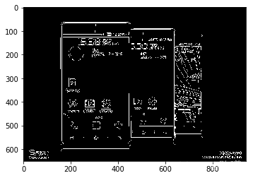
plt.imshow(edges,cmap='gray')

<matplotlib.image.AxesImage at 0x7f705843da90>
在这里插入图片描述

4.Hough直线检测（设置参数，检测对该应用有意义的直线）

# Define the Hough transform parameters
# Make a blank the same size as our image to draw on
rho = 1
theta = np.pi/180
threshold = 120
min_line_length = 100
max_line_gap = 1

line_image = np.copy(image) #creating an image copy to draw lines on

# Run Hough on the edge-detected image
lines = cv2.HoughLinesP(edges, rho, theta, threshold, np.array([]),
                        min_line_length, max_line_gap)


# Iterate over the output "lines" and draw lines on the image copy
for line in lines:
    for x1,y1,x2,y2 in line:
        cv2.line(line_image,(x1,y1),(x2,y2),(255,0,0),5)

plt.imshow(line_image)

<matplotlib.image.AxesImage at 0x7f70583ad590>
在这里插入图片描述

5.展示Hough空间

h, angles, d = st.hough_line(edges)

print("hough space type:",type(h)," data type:",h.dtype," shape: ",h.shape," dimension: ",h.ndim," max:",np.max(h)," min:",np.min(h))
print("angles space type:",type(angles)," data type:",angles.dtype," shape: ",angles.shape," dimension: ",angles.ndim)
print("dist space type:",type(d)," data type:",d.dtype," shape: ",d.shape," dimension: ",d.ndim," max:",np.max(d)," min:",np.min(d))

print("lines type:",type(lines),lines.dtype,lines.shape,lines.ndim)
img_h=np.copy(image)

wide = edges.shape[0]
height = edges.shape[1]

import math 
hough_d = math.sqrt(wide**2 + height**2)
print("hough_d:",hough_d)

angle_step = 0.5 * np.rad2deg(np.diff(angles).mean())
d_step = 0.5 * np.diff(d).mean()
# bounds = (np.rad2deg(angles[0]) - angle_step,
#           np.rad2deg(angles[-1]) + angle_step,
#           d[-1] + d_step, d[0] - d_step)

bounds = (np.rad2deg(angles[0]) + angle_step,
          np.rad2deg(angles[-1]) - angle_step,
          d[-1] - d_step, d[0] + d_step)

print("max angle",np.rad2deg(np.max(angles)),"min angle:",np.rad2deg(np.min(angles)))
print("max d",np.max(d),d[0],"min d",np.min(d),d[-1])

hough space type: <class ‘numpy.ndarray’> data type: uint64 shape: (2287, 180) dimension: 2 max: 507 min: 0
angles space type: <class ‘numpy.ndarray’> data type: float64 shape: (180,) dimension: 1
dist space type: <class ‘numpy.ndarray’> data type: float64 shape: (2287,) dimension: 1 max: 1143.0 min: -1143.0
lines type: <class ‘numpy.ndarray’> int32 (33, 1, 4) 3
hough_d: 1142.8473213863697
max angle 89.00000000000001 min angle: -90.0
max d 1143.0 -1143.0 min d -1143.0 1143.0

f,((ax1,ax2,ax3))=plt.subplots(1,3,figsize=(20,10))
ax1.set_title('original')
ax1.imshow(image)
ax2.set_title('canny edges')
ax2.imshow(edges,cmap='gray')
ax3.set_title('Hough transform')
#ax3.imshow(np.log(1+h),cmap='gray')
#ax3.imshow(h,cmap='gray')
#ax3.imshow(np.log(1+h),extent=[0,1,0,1],cmap='gray')
ax3.imshow(np.log(1+h),extent=bounds,cmap='gray',aspect='auto')

<matplotlib.image.AxesImage at 0x7f70582f75d0>
在这里插入图片描述

这是我们这周的作业，第一次尝试发出来，有问题请大家指正QAQ