记录Tensorflow的一些使用过程

之前入门tensorflow的时候根据官方文档和一些教程写的一个入门笔记。

1．安装

网址：https://tensorflow.google.cn/
$\qquad$ TensorFlow™ 是一个开放源代码软件库，用于进行高性能数值计算。借助其灵活的架构，用户可以轻松地将计算工作部署到多种平台（CPU、GPU、TPU）和设备（桌面设备、服务器集群、移动设备、边缘设备等）。TensorFlow™ 最初是由 Google Brain 团队（隶属于 Google 的 AI 部门）中的研究人员和工程师开发的，可为机器学习和深度学习提供强力支持，并且其灵活的数值计算核心广泛应用于许多其他科学领域。
$\qquad$ SciKit-learn与TensorFlow 的主要区别是：TensorFlow 更底层。而 SciKit-learn 提供了执行机器学习算法的模块化方案，很多算法模型直接就能用
其他框架：
Pytorch：
网址：https://pytorch.org/
$\qquad$ Torch 非常适用于卷积神经网络。它的开发者认为，Torch 的原生交互界面比其他框架用起来更自然、更得心应手。其次，第三方的扩展工具包提供了丰富的递归神经网络（ RNN）模型。因为这些强项，许多互联网巨头开发了定制版的 Torch，以助力他们的 AI 研究。这其中包括Facebook、Twitter，和被谷歌招安前的 DeepMind。
Theano：
$\qquad$ Theano 在深度学习框架中是祖师级的存在。它的开发始于 2007，早期开发者包括传奇人物 Yoshua Bengio 和 Ian Goodfellow。但随着 Tensorflow 在谷歌的支持下强势崛起，Theano 日渐式微，使用的人越来越少。这过程中的标志性事件是：创始者之一的 Ian Goodfellow 放弃 Theano 转去谷歌开发 Tensorflow。
Caffe：
$\qquad$ Caffe，全称Convolutional Architecture for Fast Feature Embedding。是一种常用的深度学习框架，主要应用在视频、图像处理方面的应用上。caffe是一个清晰，可读性高，快速的深度学习框架。作者是贾扬清，加州大学伯克利的ph.D，现就职于Facebook。caffe的官网是http://caffe.berkeleyvision.org/

https://tensorflow.google.cn/install/
在这里插入图片描述

2．实现线性回归

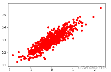
$\qquad$ 在数据上选择一条直线y=Wx+b，在这条直线上附件随机生成一些数据点如下图，让TensorFlow建立回归模型，去学习什么样的W和b能更好去拟合这些数据点。

$\qquad$ 随机生成1000个数据点，围绕在y=0.1x+0.3 周围，设置W=0.1，b=0.3，届时看构建的模型是否能学习到w和b的值。

import numpy as np
import tensorflow as tf
import matplotlib.pyplot as plt
num_points=1000    
vectors_set=[]
for i in range(num_points):
		#横坐标，进行随机高斯处理化，以0为均值，以0.55为标准差
    x1=np.random.normal(0.0,0.55)   
		#纵坐标，数据点在y1=x1*0.1+0.3上小范围浮动
    y1=x1*0.1+0.3+np.random.normal(0.0,0.03)  
    vectors_set.append([x1,y1])
    x_data=[v[0] for v in vectors_set]
    y_data=[v[1] for v in vectors_set]
    plt.scatter(x_data,y_data,c='r')
plt.show()

构造数据如下图
在这里插入图片描述

构造线性回归模型，学习上面数据图是符合一个怎么样的W和b

# 生成1维的W矩阵，取值是[-1,1]之间的随机数
W = tf.Variable(tf.random_uniform([1], -1.0, 1.0), name='W')  
# 生成1维的b矩阵，初始值是0
b = tf.Variable(tf.zeros([1]), name='b') 
# 经过计算得出预估值y
y = W * x_data + b     
# 以预估值y和实际值y_data之间的均方误差作为损失
loss = tf.reduce_mean(tf.square(y - y_data), name='loss') 
# 采用梯度下降法来优化参数  学习率为0.5
optimizer = tf.train.GradientDescentOptimizer(0.5) 
# 训练的过程就是最小化这个误差值
train = optimizer.minimize(loss, name='train')  
sess = tf.Session()
init = tf.global_variables_initializer()
sess.run(init)
# 初始化的W和b是多少
print ("W =", sess.run(W), "b =", sess.run(b), "loss =", sess.run(loss))  
for step in range(20):   # 执行20次训练
	sess.run(train)     
	# 输出训练好的W和b
	print ("W =", sess.run(W), "b =", sess.run(b), "loss =", sess.run(loss))

$\qquad$ 打印每一次结果，如下图，随着迭代进行，训练的W、b越来越接近0.1、0.3，说明构建的回归模型确实学习到了之间建立的数据的规则。loss一开始很大，后来慢慢变小，说明模型表达效果随着迭代越来越好。

W = [-0.9676645] b = [0.] loss = 0.45196822
W = [-0.6281831] b = [0.29385352] loss = 0.17074569
W = [-0.39535886] b = [0.29584622] loss = 0.07962803
W = [-0.23685378] b = [0.2972129] loss = 0.03739688
W = [-0.12894464] b = [0.2981433] loss = 0.017823622
W = [-0.05548081] b = [0.29877672] loss = 0.008751821

3. 实现CNN模型

导入TensorFlow

import tensorflow as tf
from tensorflow.examples.tutorials.mnist import input_data

加载数据集mnist
声明两个placeholder，用于存储神经网络的输入，输入包括image和label。这里加载的image是(784,)的shape。

mnist = input_data.read_data_sets('MNIST_data/', one_hot=True)
x = tf.placeholder(tf.float32,[None, 784])
y_ = tf.placeholder(tf.float32, [None, 10])

定义weights和bias

#----Weight Initialization---#
#One should generally initialize weights with a small amount of noise for symmetry breaking, and to prevent 0 gradients
def weight_variable(shape):
    initial = tf.truncated_normal(shape, stddev=0.1)
    return tf.Variable(initial)
def bias_variable(shape):
    initial = tf.constant(0.1, shape=shape)
    return tf.Variable(initial)

定义卷积层和maxpooling
为了代码的整洁，将卷积层和maxpooling封装起来。padding=‘SAME’表示使用padding，不改变图片的大小。

#Convolution and Pooling
#Our convolutions uses a stride of one and are zero padded so that the output is the same size as the input.
#Our pooling is plain old max pooling over 2x2 blocks
def conv2d(x, W):
    return tf.nn.conv2d(x, W, strides=[1,1,1,1], padding='SAME')
def max_pool_2x2(x):
    return tf.nn.max_pool(x, ksize=[1,2,2,1], strides=[1,2,2,1], padding='SAME')

tf.nn.conv2d(input, filter, strides, padding, use_cudnn_on_gpu=None, name=None)

$\qquad$ 除去name参数用以指定该操作的name，与方法有关的一共五个参数：

第一个参数input：指需要做卷积的输入图像，它要求是一个Tensor，具有[batch, in_height, in_width, in_channels]这样的shape，具体含义是[训练时一个batch的图片数量, 图片高度, 图片宽度, 图像通道数]，注意这是一个4维的Tensor，要求类型为float32和float64其中之一。
第二个参数filter：相当于CNN中的卷积核，它要求是一个Tensor，具有[filter_height, filter_width, in_channels, out_channels]这样的shape，具体含义是[卷积核的高度，卷积核的宽度，图像通道数，卷积核个数]，要求类型与参数input相同，有一个地方需要注意，第三维in_channels，就是参数input的第四维。
第四个参数padding：string类型的量，只能是"SAME","VALID"其中之一，这个值决定了不同的卷积方式
第五个参数：use_cudnn_on_gpu:bool类型，是否使用cudnn加速，默认为true。
结果返回一个Tensor，这个输出，就是我们常说的feature map，shape仍然是[batch, height, width, channels]这种形式。

reshape image数据
为了神经网络的layer可以使用image数据，我们要将其转化成4d的tensor: (Number, width, height, channels)

#To apply the layer, we first reshape x to a 4d tensor, with the second and third dimensions corresponding to image width and height,
#and the final dimension corresponding to the number of color channels.
x_image = tf.reshape(x, [-1,28,28,1])

搭建第一个卷积层
使用32个5x5的filter，然后通过maxpooling。

#----first convolution layer----#
#he convolution will compute 32 features for each 5x5 patch. Its weight tensor will have a shape of [5, 5, 1, 32].
#The first two dimensions are the patch size,
#the next is the number of input channels, and the last is the number of output channels.
W_conv1 = weight_variable([5,5,1,32])
 
#We will also have a bias vector with a component for each output channel.
b_conv1 = bias_variable([32])

#We then convolve x_image with the weight tensor, add the bias, apply the ReLU function, and finally max pool.
#The max_pool_2x2 method will reduce the image size to 14x14.
h_conv1 = tf.nn.relu(conv2d(x_image, W_conv1) + b_conv1)
h_pool1 = max_pool_2x2(h_conv1)

第二层卷积
使用64个5x5的filter。

#----second convolution layer----#
#The second layer will have 64 features for each 5x5 patch and input size 32.
W_conv2 = weight_variable([5,5,32,64])
b_conv2 = bias_variable([64])
 
h_conv2 = tf.nn.relu(conv2d(h_pool1, W_conv2) + b_conv2)
h_pool2 = max_pool_2x2(h_conv2)

构建全连接层
需要将上一层的输出，展开成1d的神经层。

#----fully connected layer----#
#Now that the image size has been reduced to 7x7, we add a fully-connected layer with 1024 neurons to allow processing on the entire image
W_fc1 = weight_variable([7*7*64, 1024])
b_fc1 = bias_variable([1024])

h_pool2_flat = tf.reshape(h_pool2, [-1, 7*7*64])
h_fc1 = tf.nn.relu(tf.matmul(h_pool2_flat,W_fc1) + b_fc1)

添加Dropout
加入Dropout层，可以防止过拟合问题。注意，这里使用了另外一个placeholder，可以控制在训练和预测时是否使用Dropout。

#-----dropout------#
#To reduce overfitting, we will apply dropout before the readout layer.
#We create a placeholder for the probability that a neuron's output is kept during dropout.
#This allows us to turn dropout on during training, and turn it off during testing.
keep_prob = tf.placeholder(tf.float32)
h_fc1_dropout = tf.nn.dropout(h_fc1, keep_prob)

输入层

#----read out layer----#
W_fc2 = weight_variable([1024,10])
b_fc2 = bias_variable([10])
y_conv = tf.matmul(h_fc1_dropout, W_fc2) + b_fc2

训练和评估
首先，需要指定一个cost function --cross_entropy，在输出层使用softmax。然后指定optimizer–adam。

#------train and evaluate----#
cross_entropy = tf.reduce_mean(tf.nn.softmax_cross_entropy_with_logits(labels=y_, logits=y_conv))
train_step = tf.train.AdamOptimizer(1e-4).minimize(cross_entropy)
accuracy = tf.reduce_mean(tf.cast(tf.equal(tf.argmax(y_, 1), tf.argmax(y_conv, 1)), tf.float32))
with tf.Session() as sess:
    tf.global_variables_initializer().run()
    for i in range(3000):
        batch = mnist.train.next_batch(50)
        if i % 100 == 0:
            train_accuracy = accuracy.eval(feed_dict = {
    
    x: batch[0],
                                                       y_: batch[1],
                                                       keep_prob: 1.})
            print('setp {},the train accuracy: {}'.format(i, train_accuracy))
        train_step.run(feed_dict = {
    
    x: batch[0], y_: batch[1], keep_prob: 0.5})
    test_accuracy = accuracy.eval(feed_dict = {
    
    x: mnist.test.images, y_: mnist.test.labels, keep_prob: 1.})
    print('the test accuracy :{}'.format(test_accuracy))
    saver = tf.train.Saver()
    path = saver.save(sess, './my_net/mnist_deep.ckpt')
    print('save path: {}'.format(path))