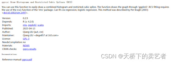
ggrcs包2.9版本发布----增加了绘制单独rcs曲线（限制立方样条）的singlercs函数

目前本人写的ggrcs包新的2.8版本已经在CRAN上线，目前支持逻辑回归（logistic回归）、cox回归和多元线性回归。增加了绘制单独rcs曲线（限制立方样条）的singlercs函数。
在这里插入图片描述
需要的可以使用代码安装

install.packages("ggrcs")

如果原来安装了旧版本，可以通过Rstudio进行升级
在这里插入图片描述

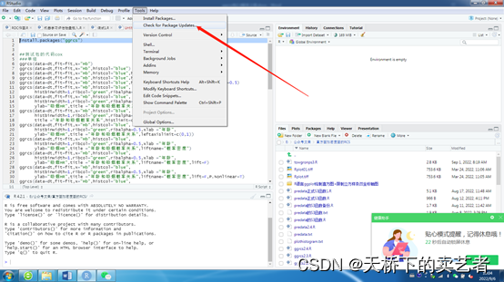
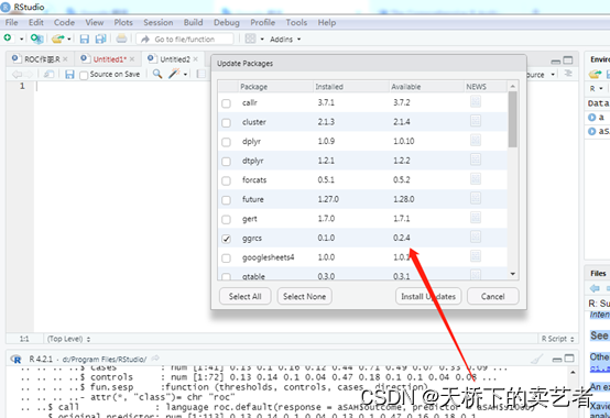
这样就可以升级到最新版本了。
部分粉丝私信给我说并不需要直方图这个密度函数，期望能出一个单独画rcs的函数，因此在2.9版本增加了singlercs函数，single就是单独单纯的意思，就是单纯画RCS，画法基本和ggrcs一样，就是没有直方图和左轴。下面我们来演示一下，只介绍新功能哈，别的功能请看既往文章。
先导入包和数据，这里使用ggrcs包自带的吸烟数据

library(rms)
library(ggplot2)
library(scales)
library(ggrcs)
dt<-smoke
dd<-datadist(dt)
options(datadist='dd')
fit<- cph(Surv(time,status==1) ~ rcs(age,4)+gender, x=TRUE, y=TRUE,data=dt)

在这里插入图片描述
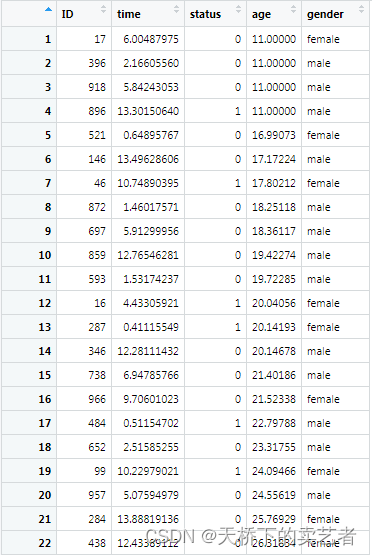
这是R包自带的吸烟数据，假设我们想了解年龄和吸烟发病率关系

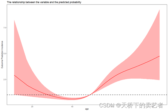
singlercs(data=dt,fit=fit,x="age")

在这里插入图片描述
本来我是在初期想加一条横线的，但是我加了后期不方便您修改，想想还是不加了，您可以生成图片后再加。这样也是挺方便的把，还方便您对线条的样式进行修改，灵活机动。

p<-singlercs(data=dt,fit=fit,x="age")
p+geom_hline(yintercept=1, linetype=2,linewidth=1)

在这里插入图片描述
您也可以使用我自写的cut.tab函数生成转折点

fit1 <-coxph(Surv(time,status==1) ~ age,data=dt)
cut.tab(fit1,"age",dt)

在这里插入图片描述
然后加上转折点虚线

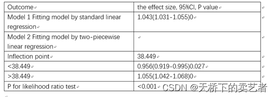
p+geom_vline(aes(xintercept=38.449),colour="#BB0000", linetype="dashed")+
  geom_hline(yintercept=1, linetype=2,linewidth=1)

在这里插入图片描述
生成转折点的表格，表明年龄在38.449岁这里发生转变，之前的OR为0.956，之后为1.055。似然比检验小于0.05表示曲线是有意义的。
cut.tab函数函数的具体用法请看《cox回归RCS阈值效应函数cut.tab1.3发布》

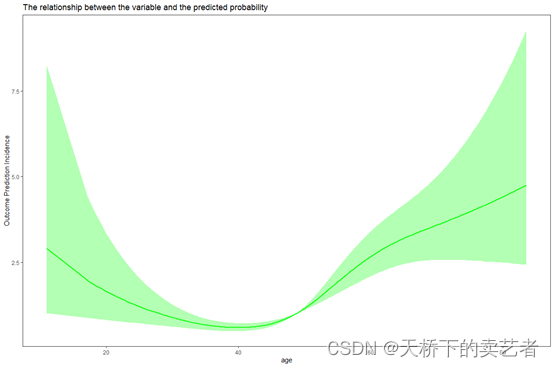
Singlercs函数还可以灵活修改，更改线条和可信区间颜色

singlercs(data=dt,fit=fit,x="age",ribcol="green")

在这里插入图片描述
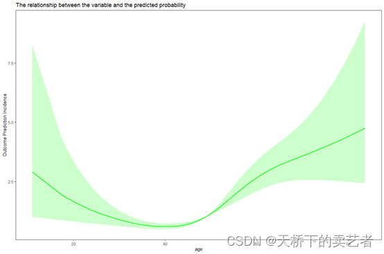
更改可信区间透明度

singlercs(data=dt,fit=fit,x="age",ribcol="green",ribalpha=0.2)

在这里插入图片描述
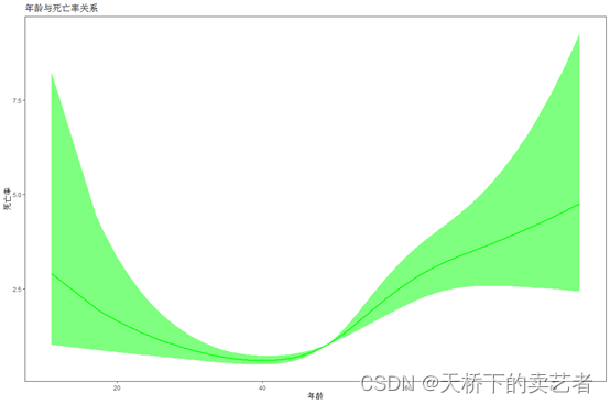
更改坐标轴和标题

singlercs(data=dt,fit=fit,x="age",histcol="blue",
          histbinwidth=1,ribcol="green",ribalpha=0.5,xlab ="年龄",ylab="死亡率",title ='年龄与死亡率关系')

在这里插入图片描述
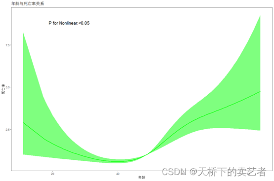
添加P值

singlercs(data=dt,fit=fit,x="age",histcol="blue",
          histbinwidth=1,ribcol="green",ribalpha=0.5,xlab ="年龄",
          ylab="死亡率",title ='年龄与死亡率关系',P.Nonlinear=T,Pvalue="<0.05")

在这里插入图片描述
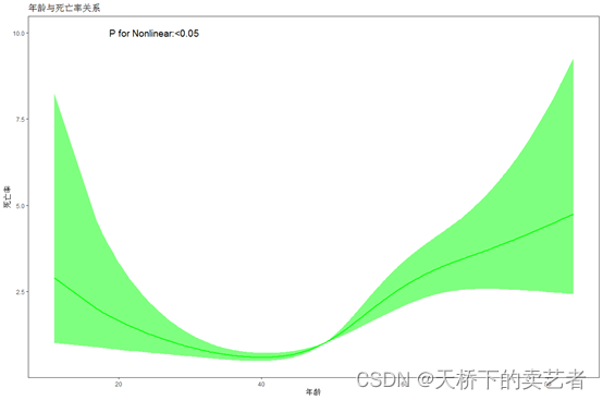
调整P值显示的位置

singlercs(data=dt,fit=fit,x="age",histcol="blue",
          histbinwidth=1,ribcol="green",ribalpha=0.5,xlab ="年龄",
          ylab="死亡率",title ='年龄与死亡率关系',P.Nonlinear=T,Pvalue="<0.05",xP.Nonlinear=25,yP.Nonlinear=10)

在这里插入图片描述
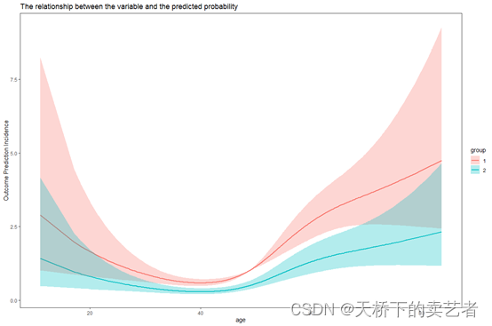
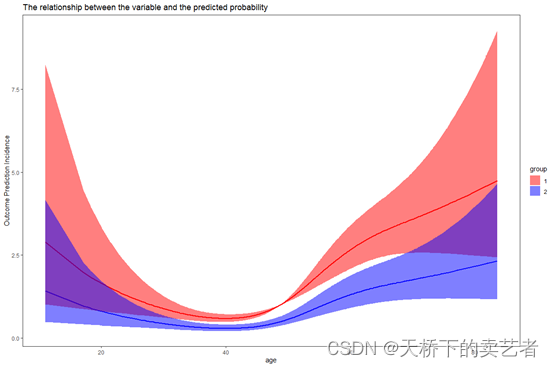
下面来介绍一下画分类（两条）RCS曲线，如果不设置颜色，默认红色和绿色

singlercs(data=dt,fit=fit,x="age",group="gender")

在这里插入图片描述
更改颜色

singlercs(data=dt,fit=fit,x="age",group="gender",groupcol=c("red","blue"))

在这里插入图片描述
更改透明度

singlercs(data=dt,fit=fit,x="age",group="gender",groupcol=c("red","blue"),ribalpha=0.5)

在这里插入图片描述
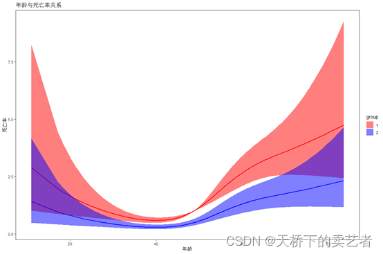
更改坐标轴和标题

singlercs(data=dt,fit=fit,x="age",group="gender",groupcol=c("red","blue"),ribalpha=0.5,
          xlab ="年龄",ylab="死亡率",title ='年龄与死亡率关系')

在这里插入图片描述
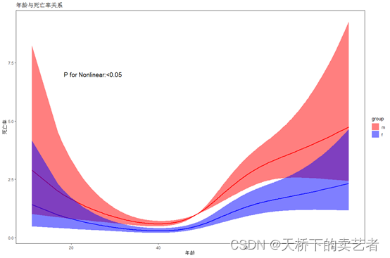
添加P值并修改P值在图片的位置

singlercs(data=dt,fit=fit,x="age",group="gender",groupcol=c("red","blue"),ribalpha=0.5,
          xlab ="年龄",ylab="死亡率",title ='年龄与死亡率关系',P.Nonlinear=T,Pvalue="<0.05",
          xP.Nonlinear=25,yP.Nonlinear=7)

在这里插入图片描述
更改标签名字

singlercs(data=dt,fit=fit,x="age",group="gender",groupcol=c("red","blue"),ribalpha=0.5,
          xlab ="年龄",ylab="死亡率",title ='年龄与死亡率关系',P.Nonlinear=T,Pvalue="<0.05",
          xP.Nonlinear=25,yP.Nonlinear=7,twotag.name= c("m","f"))

在这里插入图片描述
好了，新版本就介绍到这里了，我这里介绍了cox回归模型。逻辑回归和线性回归的做法也是一样的，值得一提的是，因为不需要画密度图，singlercs函数画线性回归的rcs比ggrcs画得好，如果使用ggrcs做线性回归rcs曲线不理想，可以考虑一下使用singlercs函数。
如果有什么建议或者R包有什么错误，欢迎你来告诉我。

ggrcs包2.9版本发布----增加了绘制单独rcs曲线（限制立方样条）的singlercs函数

猜你喜欢