# 下载skimage
pip install scikit-image -i http://pypi.douban.com/simple/ --trusted-host pypi.douban.com
一、ipython 的安装
#安装ipython
pip install ipython
# 进入ipython命令行
ipython
二、jupyter notebook的安装与配置
jupyter notebook 是一款书写python代码并可以保存运行结果的笔记工具,十分便捷。
1. jupyter的安装与启动
# 安装jupyter
pip install jupyter
# 启动jupyter-notebook
jupyter notebook
2. jupyter notebook的常用配置
jupyter notebook 的默认文件保存位置一般在C盘,而我们一般不希望将.ipynb笔记文件保存在C盘,所以,我们需要定制文件的保存位置。
- 进入命令窗口,输入
jupyter notebook --generate-config生成配置文件,生成的配置文件一般在C:\Users\liulusheng\.jupyter文件夹下的jupyter_notebook_config.py中。
# 生成jupyter notebook的配置文件
jupyter notebook --generate-config
- 找到该配置文件,用编辑器打开,找到
c.NotebookApp.notebook_dir并将注释打开,替换成需要保存到的路径即可。
c.NotebookApp.notebook_dir = 'D:\jupyter-notebook'
- 重新启动 jupyter notebook 即可。
# 启动 jupyter notebook
jupyter notebook

三、matplotlib 的使用
1. 绘制折线图
1.1 基本使用
# 引入matplotlib中的pyplot
from matplotlib import pyplot as plt
# 引入matplotlib中的font_manager
from matplotlib import font_manager

# 生成x轴的数据,需要是一个可迭代序列
x = range(2, 24, 2)

# 生成y轴的数据,需要是一个可迭代序列
y = [1, 2, 12, 34, 2, 5,6,7,8,0,9.1]

# 设置图像的宽高为20和8,每英寸的像素为90
plt.figure(figsize=(20, 8), dpi=90)

# 设置中文字体
font = font_manager.FontProperties(fname="C:\Windows\Fonts\msyh.ttc")

# 绘制图像并设置标签,且指定线条颜色为橙色
plt.plot(x, y, label="3月份", color="orange")

# 设置图例(需要和上面的label属性结合使用)
plt.legend(loc="upper left", prop=font)

# 添加网格
plt.grid(alpha=0.3)

# 添加描述信息
plt.xlabel("时间/h", fontproperties=font)
plt.ylabel("温度/℃", fontproperties=font)
plt.title("武汉市温度变化表", fontproperties=font)

# 展示图像
plt.show()

1.2 设置图片大小及清晰度
# 设置宽高为20和8,以及每英寸的像素点为100
plt.figure(figsize=(20, 8), dpi=100)
1.3 保存生成的图像
# 保存图片
plt.savefig('./demo.svg')
1.4 设置中字体
# 引入matplotlib中的font_manager
from matplotlib import font_manager
# 设置中文字体
font = font_manager.FontProperties(fname="C:\Windows\Fonts\msyh.ttc")
1.5 添加描述信息
# 添加描述信息
plt.xlabel("时间/h", fontproperties=font)
plt.ylabel("温度/℃", fontproperties=font)
plt.title("武汉市温度变化表", fontproperties=font)
1.6 设置图例
# 设置中文字体
font = font_manager.FontProperties(fname="C:\Windows\Fonts\msyh.ttc")
# 绘制图像并设置标签
plt.plot(x, y, label="3月份")
# 设置图例(需要和上面的label属性结合使用)
plt.legend(loc="upper left", prop=font)
1.7 设置网格
# 绘制图像的网格(有利于观察数据)
plt.grid(alpha=0.3)
2. 绘制散点图
绘制3月份和10月份的气温变化散点图
from matplotlib import pyplot as plt
from matplotlib import font_manager

# 3月份每天的温度
y_3 = [11, 17, 16, 11, 12, 11, 12, 6, 6, 7, 8, 9, 12, 15, 14, 17, 18, 21, 16, 17, 20, 14, 15, 15, 15, 19, 21, 22, 22.12, 26, 18]
# 10月份每天的温度
y_10 = [26, 26, 28, 19, 21, 17, 16, 19, 18, 20, 20, 19, 22, 23, 17, 20, 21, 20, 22, 15, 11, 15, 5, 13, 17, 10, 11, 15, 16, 31, 28]
# 设置图像大小
plt.figure(figsize=(20, 8), dpi=80)

# 设置字体
font = font_manager.FontProperties(fname="C:\Windows\Fonts\msyh.ttc")

x_3 = range(1, 32)
x_10 = range(41, 72)

# 绘制图像
plt.scatter(x_3, y_3, label="3月份")
plt.scatter(x_10, y_10, label="10月份")

# 设置图例
plt.legend(loc="upper left", prop=font)

# 设置x的刻度
x_ticks = list(x_3) + list(x_10)
x_labels = ["3月{}日".format(i) for i in x_3]
x_labels += ["10月{}日".format(i - 40) for i in x_10]
plt.xticks(ticks=x_ticks[::3], labels=x_labels[::3], fontproperties=font, rotation=45)

# 添加描述
plt.xlabel("日期/月日", fontproperties=font)
plt.ylabel("温度/℃", fontproperties=font)
plt.title("3月和10月的温度变化表", fontproperties=font)
# 保存该图像
plt.savefig('./scatter.svg')

# 显示图像
plt.show()

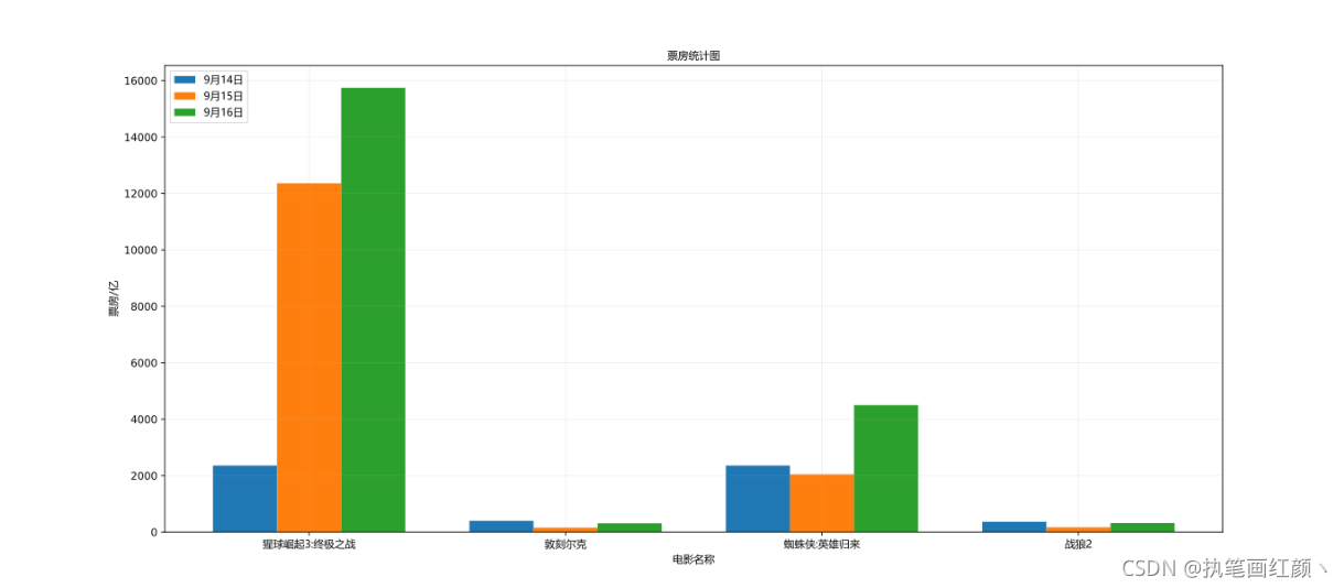
3. 绘制条形图
绘制四部热门电影分别在9月14日、9月15日、9月16日的票房数量
from matplotlib import pyplot as plt
from matplotlib import font_manager

# 四部电影的名称
a = ["猩球崛起3:终极之战", "敦刻尔克", "蜘蛛侠:英雄归来", "战狼2"]

# 14日四部电影的票房
y_14 = [2358, 399, 2358, 362]
# 15日四部电影的票房
y_15 = [12357, 156, 2045, 168]
# 16日四部电影的票房
y_16 = [15746, 312, 4497, 319]

# 设置图像的大小
plt.figure(figsize=(20,9), dpi=80)

# 设置中文字体
font = font_manager.FontProperties(fname="C:\Windows\Fonts\msyh.ttc")

# 统一设置条形柱的宽度
x_width = 0.25

# 生成x轴的数据
x_14 = range(len(a))
# [0, 1, 2, 3]
x_15 = [i+x_width for i in x_14]
# [0.25, 1.25, 2.25, 3.25]
x_16 = [i+2*x_width for i in x_14]
# [0.5, 1.5, 2.5, 3.5]

# 绘制图像
plt.bar(x_14, y_14, width=x_width, label="9月14日")
plt.bar(x_15, y_15, width=x_width, label="9月15日")
plt.bar(x_16, y_16, width=x_width, label="9月16日")

# 添加图例(与上述的label结合使用)
plt.legend(loc="upper left", prop=font)

# 设置x轴的刻度
plt.xticks(ticks=x_15, labels=a, fontproperties=font)

# 添加描述信息
plt.title("票房统计图", fontproperties=font)
plt.xlabel("电影名称", fontproperties=font)
plt.ylabel("票房/亿", fontproperties=font)

# 添加网格,有利于观察数据
plt.grid(alpha=0.2)

# 保存图像
plt.savefig('./bar.svg')

plt.show()
四、numpy 的使用
1. numpy 基本使用
1.1 生成numpy数组
# 生成numpy.ndarray的三种方式
# 方式一
t1 = np.array(range(10))
print(t1)
[0 1 2 3 4 5 6 7 8 9]
print(t1.dtype)
int32
# 方式二
t2 = np.array([1, 2, 3, 4, 5])
print(t2)
[1 2 3 4 5]
# 方式三
t3 = np.arange(2, 18, 2)
print(t3)
[ 2  4  6  8 10 12 14 16]
1.2 指定生成数组的数据类型
# 指定生成数组的数据类型
t4 = np.array([1, 1, 0, 0, 1, 0], dtype=bool)
print(t4)
[ True  True False False  True False]
1.3 修改数组的数据类型
# 修改数组的数据类型
t5 = np.array([True, True, False, False, True, False])
t6 = t5.astype(dtype="int32")
print(t6)
[1 1 0 0 1 0]
1.4 指定数组中小数的位数
# 指定数组中小数的位数
# 生成包含小数的数组,random.random() 能够生成[0,1)的小数
t7 = np.array([random.random() for i in range(10)])
print(t7)
[0.13195263 0.65366942 0.33832589 0.84553949 0.0674462  0.9550536 0.91240518 0.50317671 0.28403965 0.98534765]
# 保留两位小数
t8 = t7.round(2)
print(t8)
[0.13 0.65 0.34 0.85 0.07 0.96 0.91 0.5  0.28 0.99]
1.5 查看与修改数组的形状
# 查看数组的形状
t9 = np.array(range(12))
print(t9)
[ 0  1  2  3  4  5  6  7  8  9 10 11]
# 当数组只有一行数据时,shape数值表示的是数组元素的个数
print(t9.shape)
(12,)

# 修改数组的形状(改为3行4列的二维数组)
t10 = t9.reshape((3, 4))
print(t10)
[[ 0  1  2  3]
 [ 4  5  6  7]
 [ 8  9 10 11]]
# 当数组是二维数组时,shape数值表示的是行数和列数
print(t10.shape)
(3, 4)
2. numpy 数组的计算
2.1 数组与数字的计算
利用了其广播性,会将数字转换成对应维度的数组,再进行计算。
# 数组与数字的计算
a = np.array([1, 2, 3, 4])
print(f"相加的结果为:{

      a + 1}")
[2 3 4 5]
print(f"相乘的结果为:{

      a * 2}")
[2 4 6 8]
print(f"乘方的结果为:{

      a ** 2}")
[ 1  4  9 16]
2.2 数组与数组的计算
# 数组与数组的计算
a = np.array([1, 2, 3, 4])
b = np.array([2, 3, 4, 5])
print(f"数组相加的结果为:{

      a + b}")
[3 5 7 9]
print(f"数组相乘的结果为:{

      a * b}")
[ 2  6 12 20]
print(f"数组乘方的结果为:{

      a ** b}")
[   1    8   81 1024]
2.3 数组(矩阵)的转置
# 数组(矩阵)的转置
print(c.T)
3. numpy 读取本地数据
测试的csv文件(demo.csv)
7426393,78240,13548,7054
94203,2651,1309,0
7426393,78240,13548,7054
94203,2651,1309,0
142819,13119,151,114115
80028,65729,1529,3598
40592,5019,57,490
142819,13119,151,11411
580028,65729,1529,35984
0592,5019,57,490
317696,9449,135,4644
79291,23935,638,1941
317696,9449,135,46447
9291,23935,638,1941
10532409,384841,7547,238496
5453,2761,33,223
751743,42272,358,325011
读取文件
# 本地csv文件所在路径
file_path = "./demo.csv"

# 读取csv文件
# dtype表示是将读取的字符转换成对应的数据类型,默认是float类型
# delimiter表示的是按什么分隔符来提取内容,默认是按空格
data = np.loadtxt(file_path, delimiter=",", dtype=int)

# 输出data的类型
print(type(data))
<class 'numpy.ndarray'>
# 输出读取的数据
print(data)
[[ 7426393    78240    13548     7054]
 [   94203     2651     1309        0]
 [ 7426393    78240    13548     7054]
 [   94203     2651     1309        0]
 [  142819    13119      151   114115]]
4. numpy 索引和切片
4.1 numpy 索引
# 生成5行8列的二维数组
data = np.arange(10, 25).reshape((3, 5))

# 输出二维数组
print(data)
[[10 11 12 13 14]
 [15 16 17 18 19]
 [20 21 22 23 24]]

# 输出数组的第一行
print(data[0])
[10 11 12 13 14]
# 输出数组的第一行第二列数据
print(data[0][1])
11
4.2 numpy 切片
# 生成5行8列的二维数组
data = np.arange(10, 25).reshape((3, 5))

# 输出二维数组
print(data)
[[10 11 12 13 14]
 [15 16 17 18 19]
 [20 21 22 23 24]]

# 执行切片操作时,"," 前面的表示行,"," 后面的表示列

# 输出数组第一行中的第二列和第三列
print(data[0, 1:3])
[11 12]
# 输出数组的第二列
print(data[:, 1])
[11 16 21]
# 输出数组的第二列和第三列
print(data[:, 1:3])
[[11 12]
 [16 17]
 [21 22]]
# 取不连续的行,第一行和第三行
print(data[[0, 2]])
[[10 11 12 13 14]
 [20 21 22 23 24]]
# 取不连续的列,第一列和第三列以及第四列
print(data[:, [0, 2, 3]])
[[10 12 13]
 [15 17 18]
 [20 22 23]]
5. numpy 常用方法
5.1 numpy 三目运算符
# 生成5行8列的二维数组
data = np.arange(10, 25).reshape((3, 5))
# 输出二维数组
print(data)
[[10 11 12 13 14]
 [15 16 17 18 19]
 [20 21 22 23 24]]

# 三目运算符,data中的每一个数据,如果小于20,就设置为0,否则就设置为20
t = np.where(data < 20, 0, 20)
print(t)
[[ 0  0  0  0  0]
 [ 0  0  0  0  0]
 [20 20 20 20 20]]
5.2 数组的拼接
# 准备数组数据
# 生成3行4列的数组
t1 = np.arange(12).reshape((3, 4))
print(t1)
[[ 0  1  2  3]
 [ 4  5  6  7]
 [ 8  9 10 11]]
# 生成3行2列的数组
t2 = np.arange(6).reshape((3, 2))
print(t2)
[[0 1]
 [2 3]
 [4 5]]
# 生成1行4列的数组
t3 = np.arange(4).reshape((1, 4))
print(t3)
[[0 1 2 3]]

# 数组的拼接
# 水平拼接
t4 = np.hstack((t1, t2))
print(t4)
[[ 0  1  2  3  0  1]
 [ 4  5  6  7  2  3]
 [ 8  9 10 11  4  5]]
# 垂直拼接
t5 = np.vstack((t1, t3))
print(t5)
[[ 0  1  2  3]
 [ 4  5  6  7]
 [ 8  9 10 11]
 [ 0  1  2  3]]
5.3 数组的行列交换
# 生成3行4列的数组
t1 = np.arange(12).reshape((3, 4))
print(t1)
[[ 0  1  2  3]
 [ 4  5  6  7]
 [ 8  9 10 11]]

# 数组的行交换和列交换
# 行交换(交换第1行和第3行)
t1[[0, 2], :] = t1[[2, 0], :]
print(t1)
[[ 8  9 10 11]
 [ 4  5  6  7]
 [ 0  1  2  3]]
# 列交换(交换第2列和第4列)
t1[:, [1, 3]] = t1[:, [3, 1]]
print(t1)
[[ 0  3  2  1]
 [ 4  7  6  5]
 [ 8 11 10  9]]
5.4 生成单位矩阵
import numpy as np
# 生成3*3的单位矩阵
t1 = np.eye(3)
print(t1)
[[1. 0. 0.]
 [0. 1. 0.]
 [0. 0. 1.]]
# 将t11中的数据转换成int类型
t2 = t1.astype(int)
print(t2)
[[1 0 0]
 [0 1 0]
 [0 0 1]]
五、pandas 的使用
1. Series对象
Series对象是一维的,具有索引和与其相对应的值。
# 传入一个列表,生成Series对象
ps1 = pd.Series([1, 2, 3, 4, 5])
print(ps1)
0    1
1    2
2    3
3    4
4    5
dtype: int64
# 传入一个range对象,生成Series对象
ps2 = pd.Series(range(5))
print(ps2)
0    0
1    1
2    2
3    3
4    4
dtype: int64
# 传入一个dict字典对象,其key对应生成Series对象的索引
data = {

    "name": "刘路生", "age": 10}
print(pd.Series(data))
name    刘路生
age      10
dtype: object
# 指定index的索引
ps3 = pd.Series([1, 2, 3, 4], index=list("abcd"))
print(ps3)
a    1
b    2
c    3
d    4
dtype: int64
# 修改数据的类型
ps4 = ps3.astype(float)
print(ps4)
a    1.0
b    2.0
c    3.0
d    4.0
dtype: float64
# 查看Series对象的索引和值
print(ps4.index)
print(ps4.values)
Index(['a', 'b', 'c', 'd'], dtype='object')
[1. 2. 3. 4.]
# 求和
print(ps4.sum())
10.0
2. DataFrame对象
DataFrame对象是二维的,其实就是Series的容器,其具有行索引和列索引。
# 传入一个3*3的numpy数组作为参数,生成DataFrame对象
df1 = pd.DataFrame(np.arange(9).reshape((3, 3)))
print(df1)
   0  1  2
0  0  1  2
1  3  4  5
2  6  7  8

# 指定行索引和列索引的值
df2 = pd.DataFrame(np.arange(9).reshape((3, 3)), index=list("abc"), columns=list("DEF"))
print(df2)
   D  E  F
a  0  1  2
b  3  4  5
c  6  7  8
3. DataFrame的切片和索引
loc[行,列]:适用于指定索引别名的DataFrame对象。
iloc[行,列]:适用于索引为数字的DataFrame对象。
# 传入一个3*3的numpy数组作为参数,生成DataFrame对象
df1 = pd.DataFrame(np.arange(9).reshape((3, 3)))
print(df1)
   0  1  2
0  0  1  2
1  3  4  5
2  6  7  8
# 指定行索引和列索引的值
df2 = pd.DataFrame(np.arange(9).reshape((3, 3)), index=list("abc"), columns=list("DEF"))
print(df2)
   D  E  F
a  0  1  2
b  3  4  5
c  6  7  8

# loc的使用
# 获取列索引为E的所有值,返回的是一个Series对象
ps2 = df2['E']
print(ps2)
a    1
b    4
c    7
Name: E, dtype: int32

# 获取行索引为a,列索引为E的值
print(df2.loc["a", "E"])
1

# 获取行索引为a,列索引为D和E的值,返回的是Series对象
print(df2.loc["a", ["D", "E"]])
D    0
E    1
Name: a, dtype: int32

# 获取行索引为a和b,列索引为D和E的值,返回的是DataFrame对象
print(df2.loc[["a", "b"], ["D", "E"]])
   D  E
a  0  1
b  3  4

# iloc的使用
# 获取第一列的所有值,返回的是一个Series对象
ps1 = df1[0]
print(ps1)
0    0
1    3
2    6
Name: 0, dtype: int32

# 获取第1行第2列的值
print(df1.iloc[0, 1])
1

# 获取第2行中,第1列和2列的值,返回的是一个Series对象
print(df1.iloc[1, [0, 1]])
0    3
1    4
Name: 1, dtype: int32
4. 读取外部数据
data.csv 文件
Name,Age,Number,Identity
张三,20,13334257846,研究生
李四,21,18875413624,本科生
王五,25,14258796412,博士生
赵六,21,13334257846,本科生
老王,28,14235648752,博士生
小美,16,12347859548,本科生
张三,22,15742687942,研究生
# 读取csv文件
df = pd.read_csv("data.csv")
# 查看全部内容
print(df)

# 查看前三行的内容
print(df.head(3))
  Name  Age       Number Identity
0   张三   20  13334257846      研究生
1   李四   21  18875413624      本科生
2   王五   25  14258796412      博士生

# 查看读取内容的详细信息
print(df.info())
<class 'pandas.core.frame.DataFrame'>
RangeIndex: 7 entries, 0 to 6
Data columns (total 4 columns):
 #   Column    Non-Null Count  Dtype
---  ------    --------------  -----
 0   Name      7 non-null      object
 1   Age       7 non-null      int64
 2   Number    7 non-null      int64
 3   Identity  7 non-null      object
dtypes: int64(2), object(2)
memory usage: 352.0+ bytes
None

# 查看内容的描述信息(包括均值,方差,最小值最大值等),只会统计数值型数据
print(df.describe())
             Age        Number
count   7.000000  7.000000e+00
mean   21.857143  1.458985e+10
std     3.804759  2.164474e+09
min    16.000000  1.234786e+10
25%    20.500000  1.333426e+10
50%    21.000000  1.423565e+10
75%    23.500000  1.500074e+10
max    28.000000  1.887541e+10
5. 常用数据处理方法
数据使用上述读取的数据
# 查看内容的描述信息(包括均值,方差,最小值最大值等),只会统计数值型数据
print(df.describe())
             Age        Number
count   7.000000  7.000000e+00
mean   21.857143  1.458985e+10
std     3.804759  2.164474e+09
min    16.000000  1.234786e+10
25%    20.500000  1.333426e+10
50%    21.000000  1.423565e+10
75%    23.500000  1.500074e+10
max    28.000000  1.887541e+10

# 查看Age列的平均值
print(df['Age'].mean())
21.857142857142858

# 查看Age列的方差
print(df['Age'].std())
3.8047589248453675

"""
   XXX.str.xxx()方法还有:
       -cat(和指定字符进行拼接)
       -split(按照指定字符串分隔)
       -rsplit(和split用法一致,只不过默认是从右往左分隔)
       -zfill(填充,只能是0,从左边填充)
       -contains(判断字符串是否含有指定子串,返回的是bool类型)
       更多参考博客 https://blog.csdn.net/weixin_43750377/article/details/107979607
"""
# 对Name列的每一个值看作一个字符串,对该字符串按指定格式进行切割,生成一个列表,最终结果返回一个Series对象
temp1 = df['Name'].str.split("")
print(temp1)
0    [, 张, 三, ]
1    [, 李, 四, ]
2    [, 王, 五, ]
3    [, 赵, 六, ]
4    [, 老, 王, ]
5    [, 小, 美, ]
6    [, 张, 三, ]
Name: Name, dtype: object

# 对Name列的每一个值看成一个字符串,对该字符串按指定格式进行切割,生成一个列表,并将生成的所有列表值转换成一个大列表
list2 = df['Name'].str.split("").tolist()
print(list2)
[['', '张', '三', ''], ['', '李', '四', ''], ['', '王', '五', ''], ['', '赵', '六', ''], ['', '老', '王', ''], ['', '小', '美', ''], ['', '张', '三', '']]

# 对Name列的每一个值看作一个字符串,判断该字符串是否包含张,如果是,则返回True,否则返回False,最终结果返回一个Series对象
print(df['Name'].str.contains('张'))
0    False
1    False
2    False
3    False
4    False
5    False
6    False

# 去除重复的元素,返回ndarray对象
print(df['Name'].unique())
['张三' '李四' '王五' '赵六' '老王' '小美']