我们可以在nn/modules.py中找到Detect()类,这里首先贴一下代码
class Detect(nn.Module):
    """YOLOv8 Detect head for detection models."""
    dynamic = False  # force grid reconstruction
    export = False  # export mode
    shape = None
    anchors = torch.empty(0)  # init
    strides = torch.empty(0)  # init

    def __init__(self, nc=80, ch=()):  # detection layer
        super().__init__()
        self.nc = nc  # number of classes
        self.nl = len(ch)  # number of detection layers
        self.reg_max = 16  # DFL channels (ch[0] // 16 to scale 4/8/12/16/20 for n/s/m/l/x)
        self.no = nc + self.reg_max * 4  # number of outputs per anchor
        self.stride = torch.zeros(self.nl)  # strides computed during build
        c2, c3 = max((16, ch[0] // 4, self.reg_max * 4)), max(ch[0], self.nc)  # channels
        self.cv2 = nn.ModuleList(
            nn.Sequential(Conv(x, c2, 3), Conv(c2, c2, 3), nn.Conv2d(c2, 4 * self.reg_max, 1)) for x in ch)
        self.cv3 = nn.ModuleList(nn.Sequential(Conv(x, c3, 3), Conv(c3, c3, 3), nn.Conv2d(c3, self.nc, 1)) for x in ch)
        self.dfl = DFL(self.reg_max) if self.reg_max > 1 else nn.Identity()

    def forward(self, x):
        """Concatenates and returns predicted bounding boxes and class probabilities."""
        shape = x[0].shape  # BCHW
        for i in range(self.nl):
            x[i] = torch.cat((self.cv2[i](x[i]), self.cv3[i](x[i])), 1)
        if self.training:
            return x
        elif self.dynamic or self.shape != shape:
            self.anchors, self.strides = (x.transpose(0, 1) for x in make_anchors(x, self.stride, 0.5))
            self.shape = shape

        x_cat = torch.cat([xi.view(shape[0], self.no, -1) for xi in x], 2)
        if self.export and self.format in ('saved_model', 'pb', 'tflite', 'edgetpu', 'tfjs'):  # avoid TF FlexSplitV ops
            box = x_cat[:, :self.reg_max * 4]
            cls = x_cat[:, self.reg_max * 4:]
        else:
            box, cls = x_cat.split((self.reg_max * 4, self.nc), 1)
        dbox = dist2bbox(self.dfl(box), self.anchors.unsqueeze(0), xywh=True, dim=1) * self.strides
        y = torch.cat((dbox, cls.sigmoid()), 1)
        return y if self.export else (y, x)

    def bias_init(self):
        """Initialize Detect() biases, WARNING: requires stride availability."""
        m = self  # self.model[-1]  # Detect() module
        # cf = torch.bincount(torch.tensor(np.concatenate(dataset.labels, 0)[:, 0]).long(), minlength=nc) + 1
        # ncf = math.log(0.6 / (m.nc - 0.999999)) if cf is None else torch.log(cf / cf.sum())  # nominal class frequency
        for a, b, s in zip(m.cv2, m.cv3, m.stride):  # from
            a[-1].bias.data[:] = 1.0  # box
b[-1].bias.data[:m.nc] = math.log(5 / m.nc / (640 / s) ** 2) # cls (.01 objects, 80 classes, 640 img)首先来看一下初始化的一些属性,
nc: 整数,表示图像分类问题中的类别数;nl: 整数,表示检测模型中使用的检测层数;reg_max: 整数,表示每个锚点输出的通道数;no: 整数,表示每个锚点的输出数量,其中包括类别数和位置信息;stride: 一个形状为(nl,)的张量,表示每个检测层的步长(stride);cv2: 一个 nn.ModuleList 对象,包含多个卷积层,用于预测每个锚点的位置信息;cv3: 一个 nn.ModuleList 对象,包含多个卷积层,用于预测每个锚点的类别信息;dfl: 一个 DFL(Differentiable Feature Localization)类对象,用于应用可微分几何变换,以更好地对目标框进行回归;- shape属性表示模型期望的输入形状,如果模型只接受固定形状的输入,则
self.shape存储该形状
在前向传播中,shape获取了输入张量x的形状,并保存在shape中。
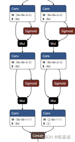
        for i in range(self.nl):
            x[i] = torch.cat((self.cv2[i](x[i]), self.cv3[i](x[i])), 1)
这里我们可以print(x[i].size())看一下,发现是:1*66*40*40,1*66*20*20,1*66*10*10,因为我是两个类,所以66 = (2+4*16)这个4*16也就是self.no = nc + self.reg_max * 4。因为我输入尺寸是320*320的,所以三个特征图是40,20,10,如果大家是640*640的,特征图应该是80,40,20。
这里同时可以打开onnx模型看一下,这一步是将cv2和cv3的输入进行concat,那么形状应该是这样:
接着如果是训练过程的话,这里的x就输出了。否则的话继续。
在这个代码片段中,self.dynamic和self.shape是两个属性,它们与输入张量的形状有关。如果 self.dynamic为真或者self.shape 与当前输入张量的形状不同,那么就会执行相应的操作。
self.dynamic属性通常用于指示模型是否支持动态形状输入。在 PyTorch 中,动态形状表示对形状进行推理,而不依赖于固定的形状尺寸。当使用动态形状时,模型可以处理任意形状的输入,并且可以通过在运行时计算形状信息来确定每个层的形状。如果模型支持动态形状输入,则 self.dynamic 属性通常设置为 True。
self.shape 属性通常用于存储模型所期望的输入形状。如果模型只接受固定形状的输入,则 self.shape 属性将存储该形状。在这种情况下,如果输入张量的形状与self.shape不匹配,则可能需要对输入进行重新调整,以适应模型的期望输入形状。
那么这个
self.anchors, self.strides = (x.transpose(0, 1) for x in make_anchors(x, self.stride, 0.5))就需要看make_anchors了,这个方法在utils/tal.py中实现:
def make_anchors(feats, strides, grid_cell_offset=0.5):
    """Generate anchors from features."""
    anchor_points, stride_tensor = [], []
    assert feats is not None
    dtype, device = feats[0].dtype, feats[0].device
    for i, stride in enumerate(strides):
        _, _, h, w = feats[i].shape
        sx = torch.arange(end=w, device=device, dtype=dtype) + grid_cell_offset  # shift x
        sy = torch.arange(end=h, device=device, dtype=dtype) + grid_cell_offset  # shift y
        sy, sx = torch.meshgrid(sy, sx, indexing='ij') if TORCH_1_10 else torch.meshgrid(sy, sx)
        anchor_points.append(torch.stack((sx, sy), -1).view(-1, 2))
        stride_tensor.append(torch.full((h * w, 1), stride, dtype=dtype, device=device))
return torch.cat(anchor_points), torch.cat(stride_tensor)feats: 一个列表,包含多个特征图;strides: 一个列表,包含多个步长;grid_cell_offset: 一个浮点数,表示每个网格单元的偏移量,默认为 0.5。
在实现中,首先遍历输入的特征图和步长,并分别获取它们的高度、宽度和步长值。然后,使用 PyTorch 的 arange() 函数生成一组横向和纵向的位移值,并添加一个偏移量(即 grid_cell_offset)以将锚点的中心对准每个网格单元的中心。
接下来,使用 PyTorch 的 meshgrid() 函数生成所有可能的锚点位置,并将其保存在 anchor_points 列表中。其中,每个锚点的位置由两个坐标值表示,即 (x, y),并被转换为形状为 (n, 2) 的张量,其中 n 表示特征图上的像素点数量。
同时,在每个特征图上都需要保存相应的步长信息,以便后续计算。因此,使用 PyTorch 的 full() 函数创建一个形状为 (h*w, 1) 的张量,其中 h 和 w 分别表示特征图的高度和宽度,每个元素都被初始化为当前特征图的步长值。
最终,通过将所有锚点位置和步长信息连接起来,可以得到形状为 (n*nl, 2) 和 (n*nl, 1) 的张量,其中 nl 表示特征图的数量,n 表示每个特征图上的像素点数量。这些张量将被用于计算每个锚点的位置和预测信息,并生成最终的预测结果。
所以经过transpose后,得到的anchor应该是(2,2100),stride是(1,2100)
三个x[i]进行concat:
x_cat = torch.cat([xi.view(shape[0], self.no, -1) for xi in x], 2)得到的x_cat的size()应该是1*66*2100,因为xi.view(shape[0],self.no,-1)中的-1表示根据其他维度的值组合成一维,即40*40=1600,20*20=400,10*10=100。
下一步的if else其实输出是一样的(我是这么认为的,若有错误请指点)
都是将x_cat的第二个维度66分成box的64和cls的2,这里的box的第二个维度经过dfl的操作变成4维的1*4*2100,与升维后的anchors.unsqueeze(0)送入dist2bbox进行计算,得到xywh值。
这里贴一下dist2bbox的实现:
def dist2bbox(distance, anchor_points, xywh=True, dim=-1):
"""Transform distance(ltrb) to box(xywh or xyxy)."""
lt, rb = distance.chunk(2, dim)
#print('lt:',lt.size())
#print('rb:',rb.size())
x1y1 = anchor_points - lt
x2y2 = anchor_points + rb
if xywh:
c_xy = (x1y1 + x2y2) / 2
wh = x2y2 - x1y1
return torch.cat((c_xy, wh), dim) # xywh bbox
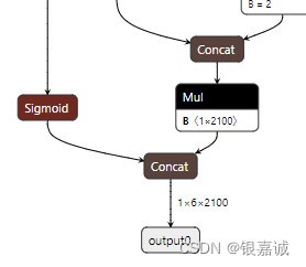
return torch.cat((x1y1, x2y2), dim) # xyxy bbox这里lt和rb分别代表x y w h的偏移量。
紧接着y = torch.cat((dbox, cls.sigmoid()), 1),将xywh和经过sigmoid归一化后的2个cls在第二维度上进行组合,形成了最终的1*6*2100,也就是最终的output。
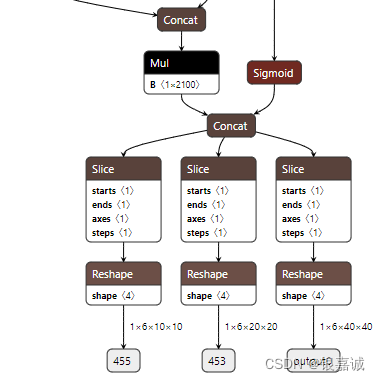
在这里向大家提一个问题,如果我想把1*6*2100的输出,拆成三个特征图的输出,直接view()是否可行呢,也就是如此:
        y1 = y[:,:,:1600]
        y2 = y[:,:,1600:2000]
        y3 = y[:,:,2000:]
        y1 = y1.view(1, 6, 40, 40)
        y2 = y2.view(1, 6, 20, 20)
        y3 = y3.view(1, 6, 10, 10)
        #print(y1.size())
        #print(y2.size())
        return  y1, y2, y3 if self.export else (y, x)