Exercise 4.2

Exercise 4.3

(4.2)Policy Improvement

0. 前言

Sutton-book第4章（动态规划）学习笔记。本文是关于其中4.1节（策略估计）和4.2节（策略提升）。

当给定MDP的完全模型后，可以基于动态规划算法求解最优策略。

经典的动态规划算法理论意义重大，但是其局限性在于：

要求MDP模型完全已知
运算量巨大

事实上，所有使用的强化学习算法都可以看作是动态规划算法的近似。

DP可以用于连续强化学习问题，但是仅限于有限的特殊情况能够给出精确解。常见的做法是将连续问题离散化，然后基于有限MDP的动态规划方法求解。

问题设定：Finite MDP{S, A, R, p(s’,r|s,a)}

Key Idea：基于价值函数进行结构化的策略搜索。

在第3章中提到，最优策略满足最优贝尔曼方程：

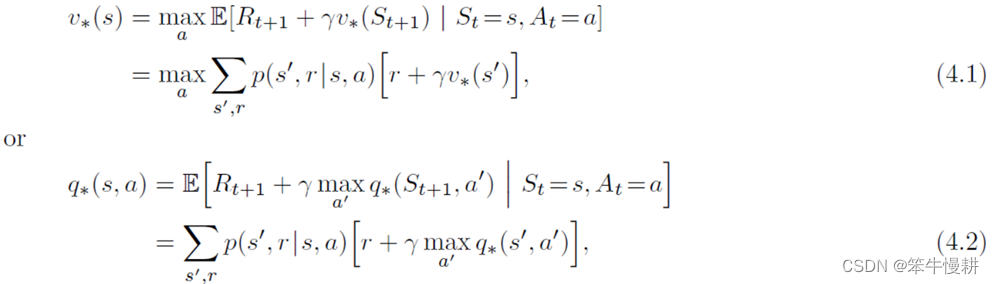
将以上贝尔曼最优方程略作修改，从方程改为递归式赋值（更新）即得到对应的动态规划算法（如以下式(4.5)所示）！

(4.1)策略估计，Policy Evaluation(Prediction)

简而言之，策略估计（或者说预测）就是指基于策略\pi(a|s)求对应的状态值函数：

如果环境动力学函数(env dynamics) $p(s',r|s,a)$ 已知的话，上式其实就是一个线性方程组（未知数个数=|S|），可以直接求解。当然更实际的方式是用迭代的方式求解，迭代更新规则（update rule）可以由（4.4）简单地改写而来：

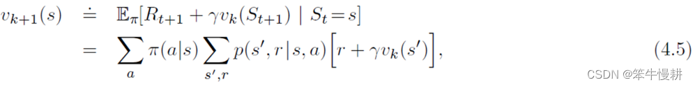
该迭代方程的不动点即是(4.4)的解。

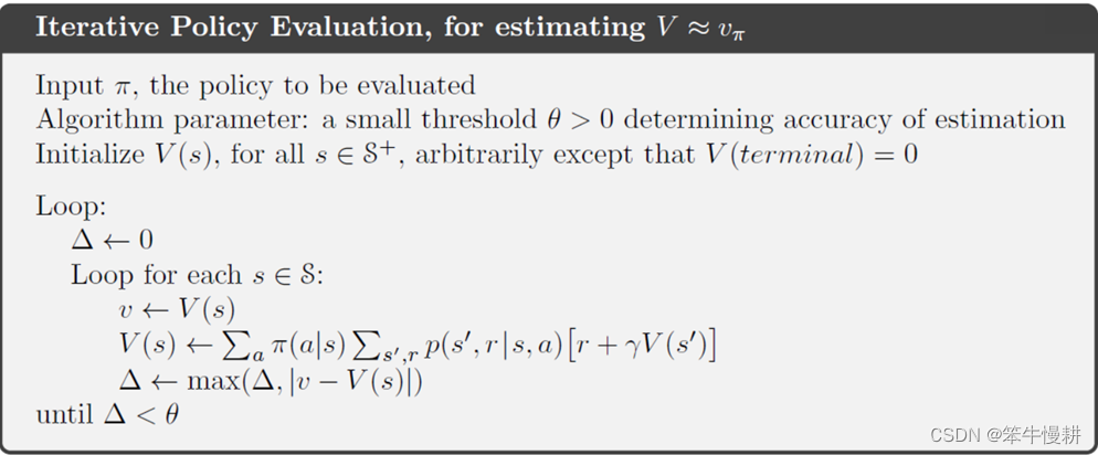
迭代式策略评价的处理流程（伪代码）如下所示：

Some key-points:

迭代终止条件
In-place update or not. In-place是指一个状态的新值被计算出来后立即更新用于同一次迭代中的后续状态的更新；与之相对的是，所有状态的值在一轮迭代结束后同时被更新。前者收敛速度通常更快。但是，在in-place算法中，状态更新顺序对于收敛速度有很大的影响。

Example 4.1 (python代码)

Consider the 4x4 gridworld shown below.

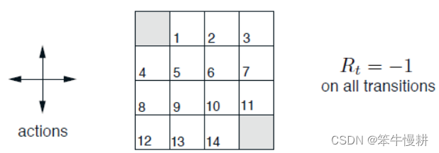
非终止状态集（non-terminal states set） is $\mathcal{S} = [1,2,...,14]$ . 左上角和右下角为终止状态。

在非终止状态，等概率采取{上，下，左，右}动作之一。每次移动（状态转移）的即时奖励都是-1。如果在某状态下采取某个行动导致移出了以上gridworld则退回原地（但是仍然产生-1的即时奖励）。

基于迭代的方式求解以上游戏的状态价值的python代码如下所示：

# -*- coding: utf-8 -*-
"""
Created on Sat Feb  4 15:46:15 2023

@author: chenxy
"""
import numpy as np

states  = [      (0,1),(0,2),(0,3), 
           (1,0),(1,1),(1,2),(1,3), 
           (2,0),(2,1),(2,2),(2,3), 
           (3,0),(3,1),(3,2)        ]                 
s_term  = tuple([(0,0),(3,3)]) # Terminal states

actions = ['UP','DOWN','LEFT','RIGHT']
def policy(s,a):
    '''
    The agent follows the equiprobable random policy (all actions equally likely).
    '''
    prob_s_a = 1.0 / len(actions)
    
    return prob_s_a

def transit_to(s,a):
    '''
    next_state to which when taking action "a" from the current state "s"
    '''
    s_next = list(s)
    if a == 'UP':
        s_next[0] = s[0] - 1
    elif a == "DOWN":
        s_next[0] = s[0] + 1
    elif a == "LEFT":
        s_next[1] = s[1] - 1
    else:
        s_next[1] = s[1] + 1
    
    if s_next[0] < 0 or s_next[0] > 3 or s_next[1] < 0 or s_next[1] > 3:
        s_next = list(s)
    
    return tuple(s_next)

def reward_func(s):
    '''
    The immediate reward when transit from other states to this state.
    Reward is -1 for all transitions.
    '''
    # return 0 if s in s_term else -1
    return -1


# Initialize v(s) to all-zeros
v = np.zeros((4,5))

iter_cnt = 0    
while True:
    max_delta = 0    
    for (i,j) in states:
        s = (i,j)
        new_v = 0
        for a in actions:
            p_action = policy(s,a)
            s_next   = transit_to(s,a)
            reward   = reward_func(s_next)
            new_v    = new_v + p_action * (reward + v[s_next[0],s_next[1]])
            
        max_delta= max(max_delta, abs(new_v - v[i][j]))
        v[i][j] = new_v
    iter_cnt = iter_cnt + 1
    # print('iter_cnt = {0}, max_delta = {1}, v = {2}'.format(iter_cnt, max_delta, v))
    if max_delta < 0.001 or iter_cnt == 100:        
        break

# How to specify format when printing np numeric array?
print('iter_cnt = {0},  v = \n {1}'.format(iter_cnt, v))

运行结果如下（解除其中的注释语句可以得到中间每次迭代后的价值变化情况）：

iter_cnt = 88, v =
[[ 0. -13.99330608 -19.99037659 -21.98940765 0. ]
[-13.99330608 -17.99178568 -19.99108113 -19.99118312 0. ]
[-19.99037659 -19.99108113 -17.99247411 -13.99438108 0. ]
[-21.98940765 -19.99118312 -13.99438108 0. 0. ]]

Exercise 4.1

In Example 4.1, if $\pi$ is the equiprobable random policy, what is $q_{\pi}(11, down)$ ?
What is $q_{\pi}(7, down)$ ?

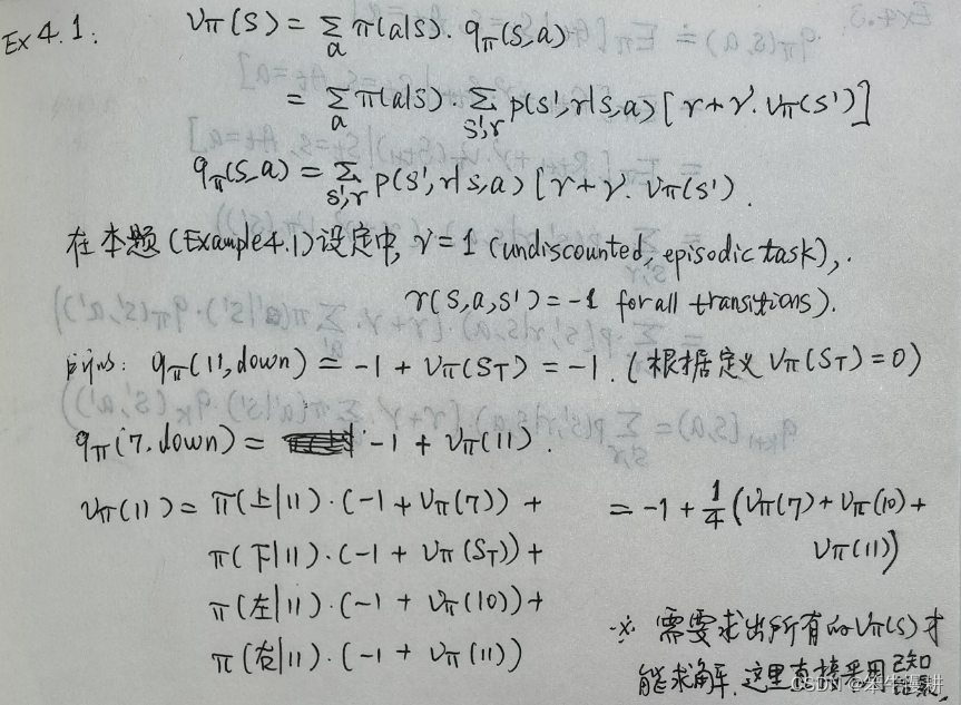
由以上Example4.1的计算已经得到 $v_{\pi}(14)=-14$ ，因此可以得到 $q_{\pi}(7,down) = -15$ .

Exercise 4.2

In Example 4.1, suppose a new state 15 is added to the gridworld just below state 13, and its actions, left, up, right, and down, take the agent to states 12, 13, 14, and 15, respectively. Assume that the transitions from the original states are unchanged. What, then, is $v_{\pi}(15)$ for the equiprobable random policy? Now suppose the dynamics of state 13 are also changed, such that action down from state 13 takes the agent to the new state 15. What is $v_{\pi}(15)$ for the equiprobable random policy in this case?

这里采用直接仿真的方法来求解。在以上Example4.1的代码的基础上稍作修改。首先是状态集合的修改（追加状态15，即如下所示的（4，1））：

states  = [      (0,1),(0,2),(0,3), 
           (1,0),(1,1),(1,2),(1,3), 
           (2,0),(2,1),(2,2),(2,3), 
           (3,0),(3,1),(3,2)      ,
                 (4,1)             ]

然后是状态转移函数的修改。以下transit_to_1对应于第1小问，即状态13在采用行动DOWN时仍然保持在原地；transit_to_2对应于第2小问，即状态13在采用行动DOWN时转移到状态15。

def transit_to_1(s,a):
    '''
    next_state to which when taking action "a" from the current state "s"
    Add (4,1) as state15, and its actions, left, up, right, and down, take the agent to states 12, 13, 14,
and 15, respectively.
    Assume that the transitions from the original states are unchanged.
    '''

    if s == (4,1):     
        s_next = list(s)
        if a == 'UP':
            s_next = (3,1)
        elif a == "DOWN":
            s_next = (4,1)
        elif a == "LEFT":
            s_next = (3,0)
        else:
            s_next = (3,2)
        return s_next

    # Keeps the transitions from the original states are unchanged
    s_next = list(s)
    if a == 'UP':
        s_next[0] = s[0] - 1
    elif a == "DOWN":
        s_next[0] = s[0] + 1
    elif a == "LEFT":
        s_next[1] = s[1] - 1
    else:
        s_next[1] = s[1] + 1
    
    if s_next[0] < 0 or s_next[1] < 0 or s_next[1] > 3 or s_next[0] > 3:
        s_next = list(s)
    
    return tuple(s_next)

def transit_to_2(s,a):
    '''
    next_state to which when taking action "a" from the current state "s"
    Add (4,1) as state15, and its actions, left, up, right, and down, take the agent to states 12, 13, 14,
and 15, respectively.
    Assume that the transitions from the original states are unchanged, except allowing transition from state 13 to 15
    '''
    if s == (4,1):     
        s_next = list(s)
        if a == 'UP':
            s_next = (3,1)
        elif a == "DOWN":
            s_next = (4,1)
        elif a == "LEFT":
            s_next = (3,0)
        else:
            s_next = (3,2)
        return s_next

    if s == (3,1):     
        s_next = list(s)
        if a == 'UP':
            s_next = (2,1)
        elif a == "DOWN":
            s_next = (4,1)
        elif a == "LEFT":
            s_next = (3,0)
        else:
            s_next = (3,2)
        return s_next
    
    s_next = list(s)
    if a == 'UP':
        s_next[0] = s[0] - 1
    elif a == "DOWN":
        s_next[0] = s[0] + 1
    elif a == "LEFT":
        s_next[1] = s[1] - 1
    else:
        s_next[1] = s[1] + 1
    
    if s_next[0] < 0 or s_next[1] < 0 or s_next[1] > 3 or s_next[0] > 3:
        s_next = list(s)
    
    return tuple(s_next)

相应地价值函数需要初始化为（5x4）的数组，如下所示：

v = np.zeros((5,4))

采用transit_to_1转移函数时的运行结果如下所示：

iter_cnt = 88, v =
[[ 0. -13.99330608 -19.99037659 -21.98940765]
[-13.99330608 -17.99178568 -19.99108113 -19.99118312]
[-19.99037659 -19.99108113 -17.99247411 -13.99438108]
[-21.98940765 -19.99118312 -13.99438108 0. ]
[ 0. -19.9913949 0. 0. ]]

采用transit_to_2转移函数时的运行结果如下所示：

iter_cnt = 88, v =
[[ 0. -13.99368565 -19.99091139 -21.98998828]
[-13.99371792 -17.99227921 -19.99159794 -19.99168042]
[-19.99099732 -19.99166012 -17.99293986 -13.99471074]
[-21.99012528 -19.99182947 -13.994762 0. ]
[ 0. -19.99199263 0. 0. ]]

可以看到，以上两种变更对于原始的状态1~状态14的价值几乎没有影响。而且这两种变更之间新增的状态15的价值估计也没有差异。为什么呢？

首先考虑第1小问。由于原来的state1~state14的行为不变（它们不会转移到状态15去），新增的state15的行为对于state1~state14的价值没有任何影响（记住，状态值贝尔曼方程对应着back-up diagram，只有在状态转移树的下游（后代）节点会对当前节点的价值产生影响）。

其次考虑第2小问。相比第1小问，其变化在于允许state13在采取行动DOWN时会转移到state15。。。嗯，容我再想象如何解释^-^

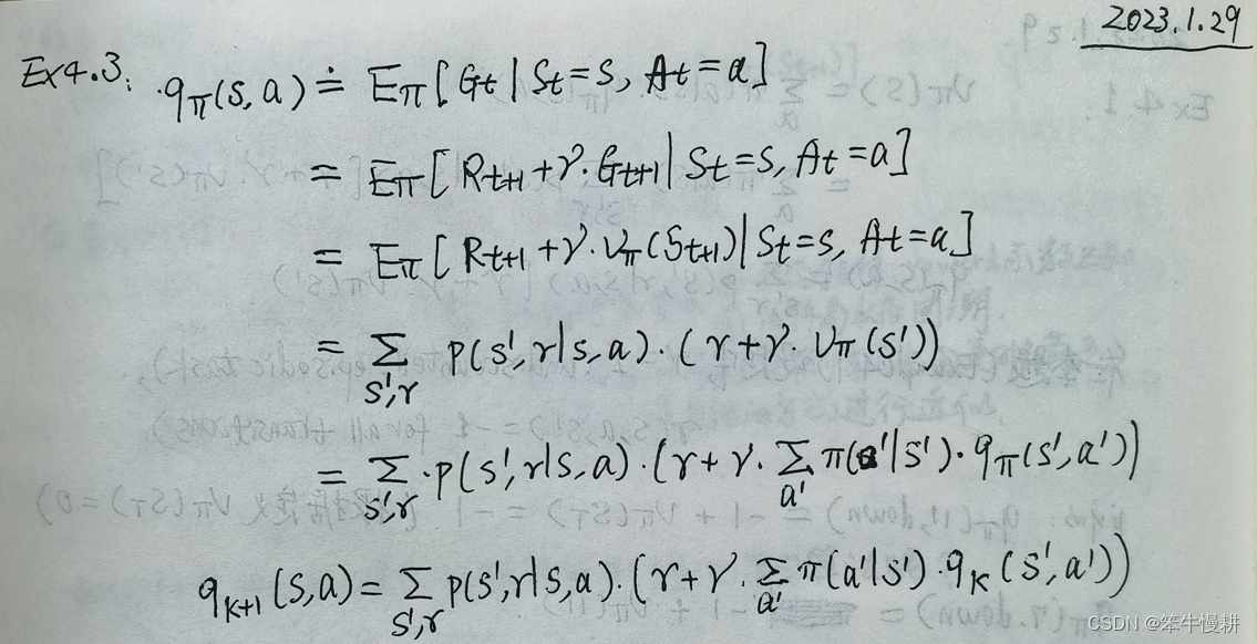
Exercise 4.3

What are the equations analogous to (4.3), (4.4), and (4.5), but for action-value
functions instead of state-value functions?

(4.2)Policy Improvement

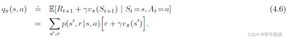
估计策略的价值函数的目的是帮助搜索好的策略。假定我们已经有了一个确定性（deterministic）策略 $\pi$ 的价值函数 $v_{\pi}$ ，现在我们想知道在状态s时到底是不是应该遵循策略 $\pi$ 来决定行动呢？可以这样来考虑，如果基于策略 $\pi$ 来决定行动，那我们已经知道了状态s的价值 $v_{\pi}(s)$ 。但是如果选择 $a \neq \pi(s)$ 呢，（假定此后仍然是按照策略 $\pi$ 行动，则）对应的状态-动作价值为：

所以当前状态s下遵循策略 $\pi$ 进行行动决策是否最优就变成了比较 $v_{\pi}(s)$ 和 $q_{\pi}(s,a)$ 的大小的问题。

一般来说，对于两个确定性策略 $\pi'$ ， $\pi$ ，如果以下不等式成立：

$\forall s \in \mathcal{S}, q_{\pi}(s, \pi'(s)) >= v_{\pi}(s) \quad (4.7)$

则必有以下不等式也成立：

$\forall s \in \mathcal{S}, v_{\pi'}(s) >= v_{\pi}(s) \quad (4.8)$

对于任何状态s，如果式(4.7)是严格大于地成立的话，式(4.8)也是严格大于地成立。

这样我们可以说策略 $\pi'$ 是优于策略 $\pi$ 的。这就是所谓的策略提升定理（policy improvement theorem）。

作为一种特殊情况，如果确定性策略 $\pi'$ 和 $\pi$ 在除状态s以外的所有情况下都相同，仅仅是在状态s下满足(4.7)和(4.8)，也仍然可以说策略 $\pi'$ 优于策略 $\pi$ 。

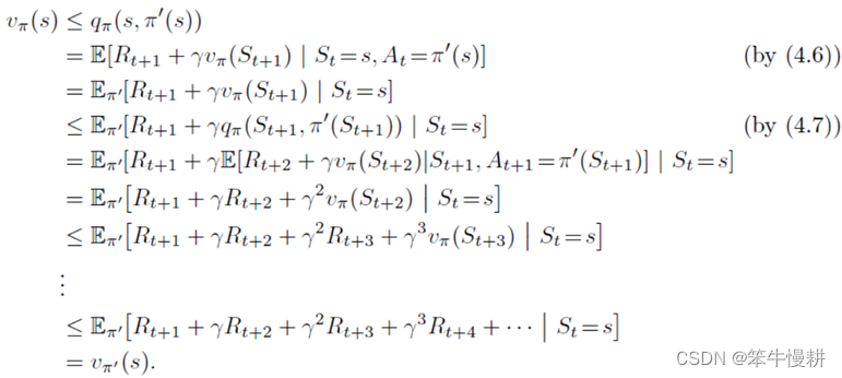
策略提升定理（式(4.7) ==> 式(4.8)）的证明如下（The idea behind the proof of the policy improvement theorem is easy to understand. Starting from (4.7), we keep expanding the q⇡ side with (4.6) and reapplying (4.7) until we get v⇡0 (s):）：

以上讨论的是在一个给定的确定性策略的条件下，评估在某个状态s下变更策略所带来的（策略）价值变化。很自然地，我们可以基于以上讨论的结论，每个状态下，基于q_{\pi}(s,a)和贪婪策略来求出对当前策略的改进策略，考虑\pi’(s)如下：

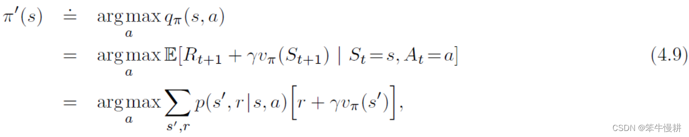
基于这个构造性定义（by construction），我们知道这个新的策略 $\pi'(s)$ 一定是满足式(4.7)和式(4.8)，因此必然是至少不比原始策略 $\pi$ 差。这种基于贪婪的方法得到策略改进的方式称之为策略提升（policy improvement）。

可以证明，只要原始策略 $\pi$ 不是满足贝尔曼最有方程的最优策略，以上策略提升过程必然可以给出（strictly）更好的策略。

以上讨论虽然是基于确定性策略进行的，但是其中的讨论过程以及结论完全可以自然地推广到随即策略。

强化学习笔记：强化学习笔记总目录

RL笔记：动态规划(1): 策略估计和策略提升

0. 前言

(4.1)策略估计，Policy Evaluation(Prediction)

Example 4.1 (python代码)

Exercise 4.1

Exercise 4.2

Exercise 4.3

(4.2)Policy Improvement

猜你喜欢